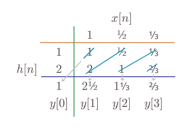
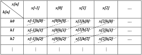
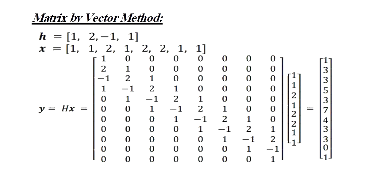
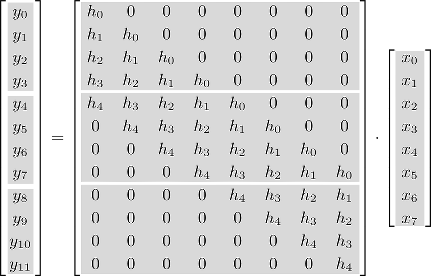
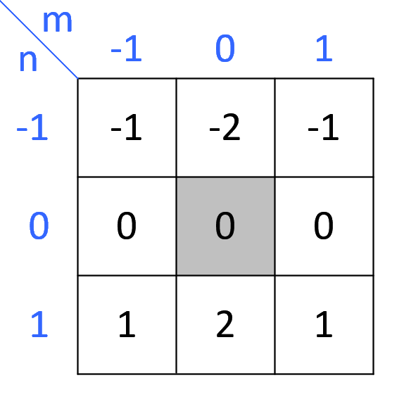
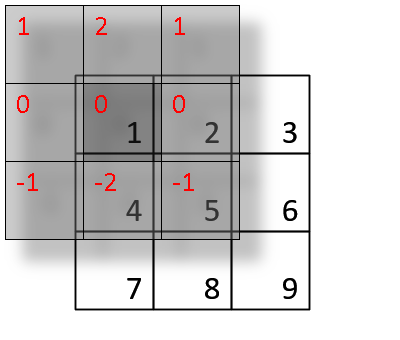
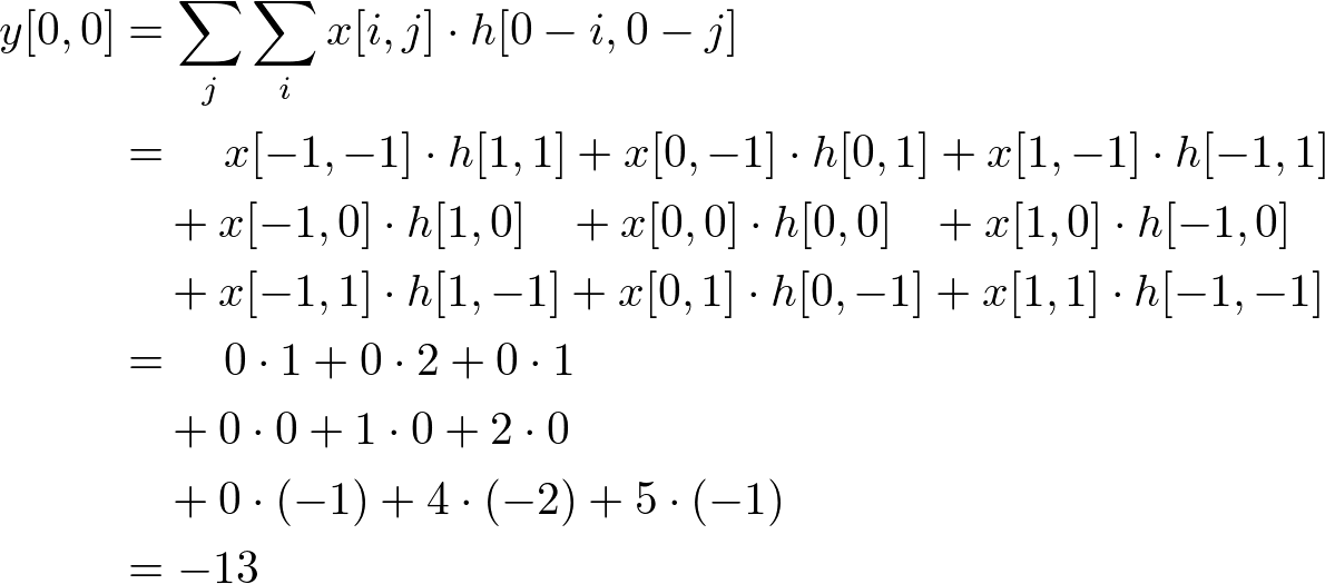
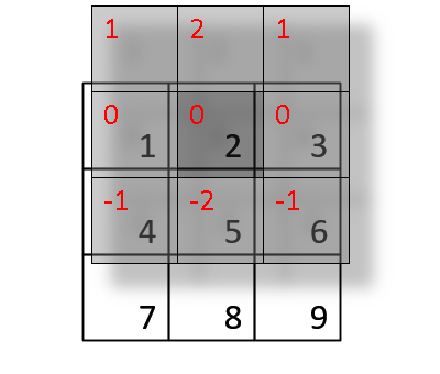
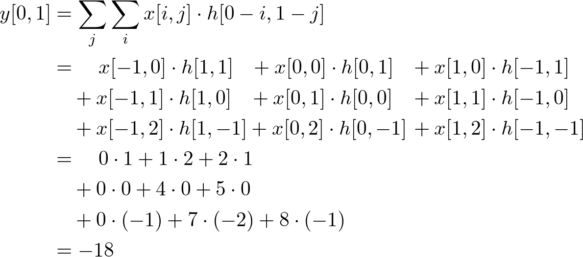
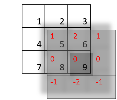
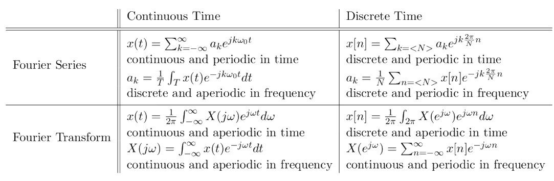
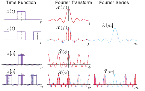
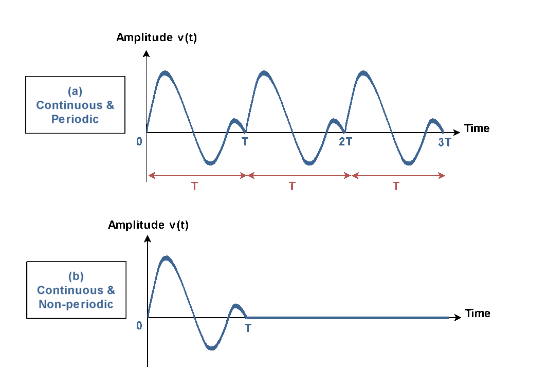
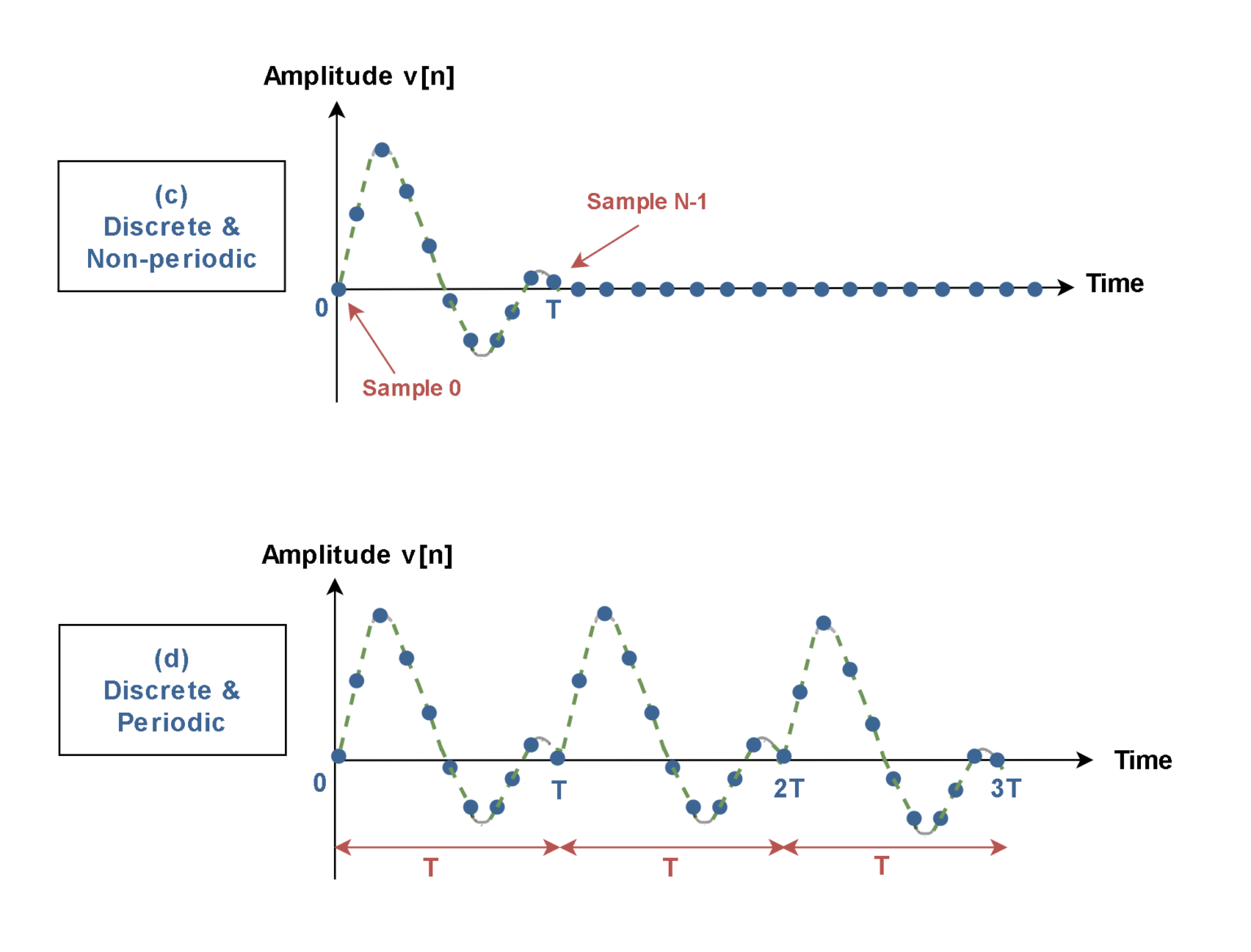
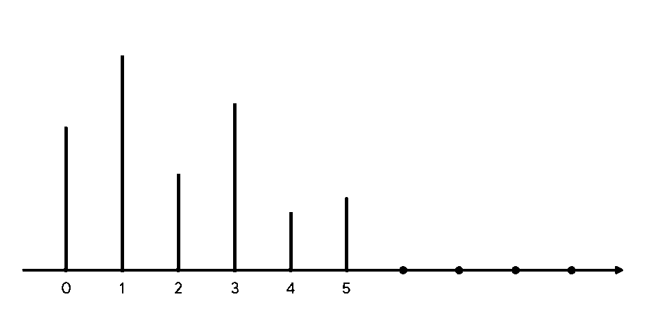
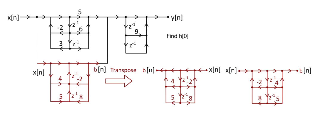
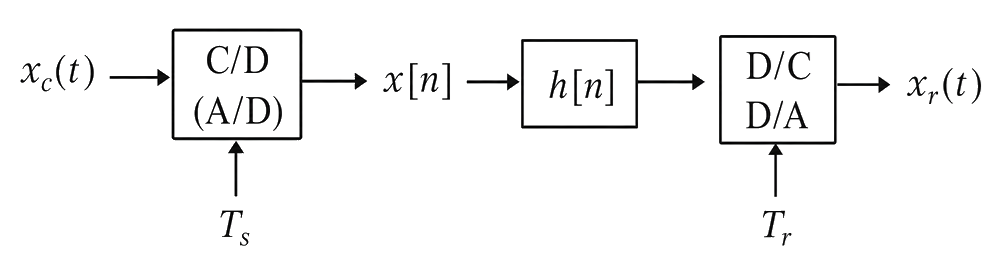
Discrete Time Processing
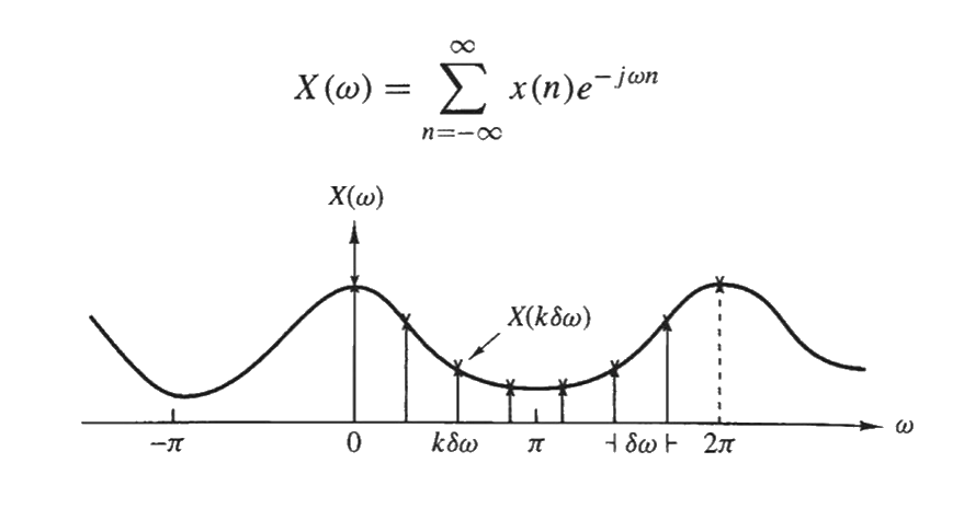
To more easily distinguish between signal frequencies and Fourier Transforms, one can use \(\omega\) in continuous time and \(\Omega\) in discrete time. In other words, a signal may have frequency component \(\omega\) in the time domain and \(\Omega\) when sampled. \(\Omega\) can be considered the “normalized” frequency relative to each sample in the discrete domain.
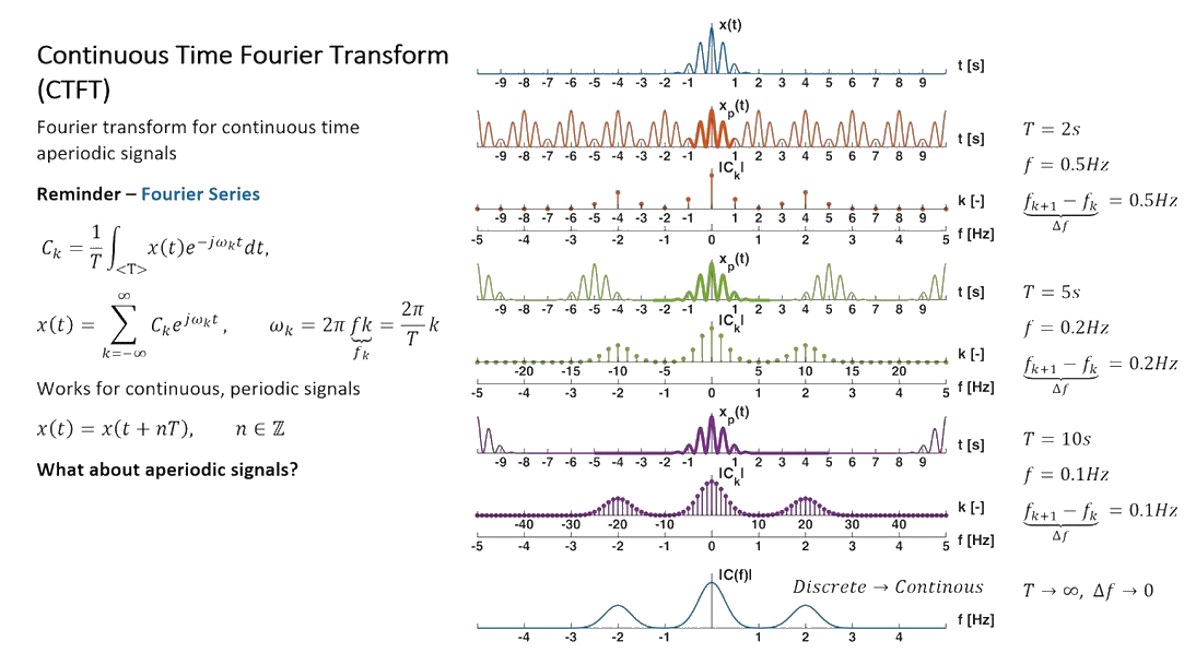
\(T\) is the sampling period such that \(\omega_s = 2 \pi / T\).
Continuous to Discrete Conversion
we can represent the Fourier Transform of a continuous time sampled signal in the \(\omega\) domain as
\[
\begin{align}
x_p(t) = \sum_{n=-\infty}^{\infty} x_c(nT) \delta(t-nT) &\stackrel{\mathcal{F}}{\leftrightarrow} X_p(j \omega) = \sum_{n=-\infty}^{\infty} x_c(nT) e^{-j \omega n T} \\
\end{align}
\]
A generic discrete time signal has the Fourier Transform in the \(\Omega\) domain as
\[
\begin{align}
x_d[n] &\stackrel{\mathcal{F}}{\leftrightarrow}
X_d(e^{j \Omega}) = \sum_{n=-\infty}^{\infty} x_d[n] e^{- j \Omega n} \\
\end{align}
\]
If we assert that this discrete time signal that relates to the continuous time signal by \(x_d[n] = x_c(nT)\) we may rewrite the Fourier Transform as
\[
\begin{align}
x_d[n] = x_c(nT) &\stackrel{\mathcal{F}}{\leftrightarrow}
X_d(e^{j \Omega}) = \sum_{n=-\infty}^{\infty} x_c(nT) e^{- j \Omega n} \\
\end{align}
\]
Note that if we substitute the relationship \(\omega = \Omega / T\) into the continuous time sampled signal \(X_p(j \omega)\), we get
\[
\begin{align}
X_p(j \Omega / T) &= \sum_{n=-\infty}^{\infty} x_c(nT) e^{-j (\Omega / T) n T} &&\omega = \Omega / T \\ \Rightarrow
X_p(j \Omega / T) &= \sum_{n=-\infty}^{\infty} x_c(nT) e^{-j \Omega n} &&\omega = \Omega / T \\
\end{align}
\]
and so, the continuous and the discrete sampled cases can be compared with
\[
\begin{align}
X_d(e^{j \Omega}) = X_p(j \Omega / T) \\
\end{align}
\]
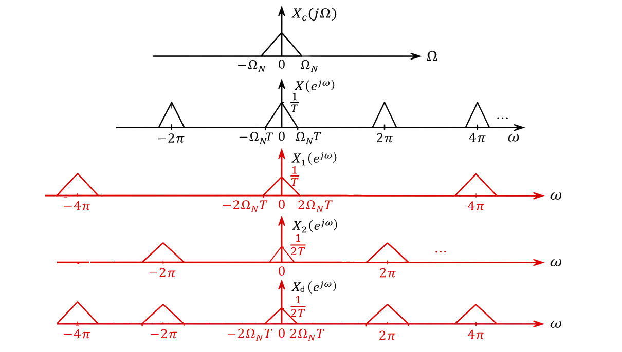
In other words, the frequency response in the continuous case at frequency \(\omega\) will correspond to the discrete frequency \(\Omega = \omega T\), and the resulting frequency response is scaled by \(T\) in the frequency axis. This relationship \(\Omega = \omega T\) is used quite frequently in subsequent analysis, and it implies the following additional relationships of note:
\((\omega)\;\frac{radians}{second}\times(T)\;seconds\;=\;(\Omega)\;radians\)
\[
\begin{align}
\omega &= \frac{\Omega}{T} \\
\omega &= \Omega f_s \\
2 \pi f &= \Omega f_s \\
\frac{f}{f_s} &= \frac{\Omega}{2 \pi} \\
\frac{\omega}{\omega_s} &= \frac{\Omega}{2 \pi} \\
\\
T &= \frac{\Omega}{\omega} \\
f_s &= \frac{\omega}{\Omega} \\
\end{align}
\]
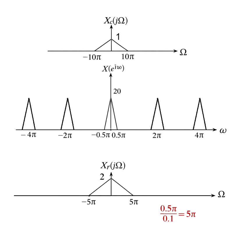
Comparing Continuous and Sampled Discrete Frequency Response
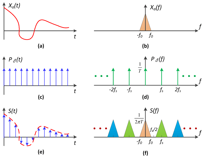
The continuous sampled signal can also be represented as a the scaled frequency response copied every \(\omega_s\), and defined by
\[
\begin{align}
x_p(t) = \sum_{n=-\infty}^{\infty} x_c(nT) \delta(t-nT) &\stackrel{\mathcal{F}}{\leftrightarrow} X_p(j \omega) = \frac{1}{T} \sum_{k=-\infty}^{\infty} X_c(j(\omega – k \omega_s)) \\
\end{align}
\]
Using the substitution \(\omega = \Omega / T\) we can also rewrite the frequency response as
\[
\begin{align}
X_p(j \Omega / T) = \frac{1}{T} \sum_{k=-\infty}^{\infty} X_c\left( j \left(\frac{\Omega}{T} – k \omega_s \right) \right) \\
\end{align}
\]
which we just found to be equivalent to \(X_d(e^{j \Omega})\) or
\[
\begin{align}
X_d(e^{j \Omega}) &= \frac{1}{T} \sum_{k=-\infty}^{\infty} X_c\left( j \left(\frac{\Omega}{T} – k \omega_s \right) \right) \\
X_d(e^{j \Omega}) &= \frac{1}{T} \sum_{k=-\infty}^{\infty} X_c\left( j \left(\frac{\Omega}{T} – k \frac{2 \pi}{T} \right) \right) \\
X_d(e^{j \Omega}) &= \frac{1}{T} \sum_{k=-\infty}^{\infty} X_c\left( j \frac{\Omega – 2 \pi k}{T}\right) \\
\end{align}
\]
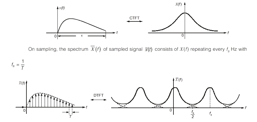
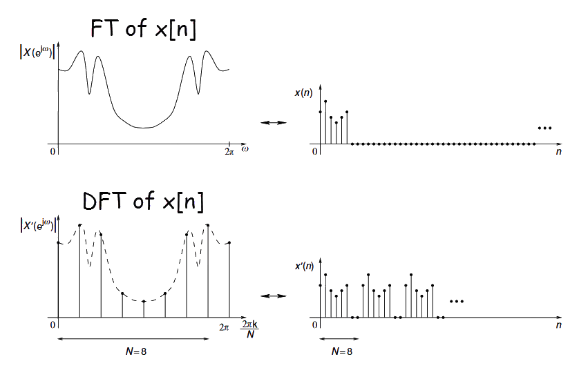
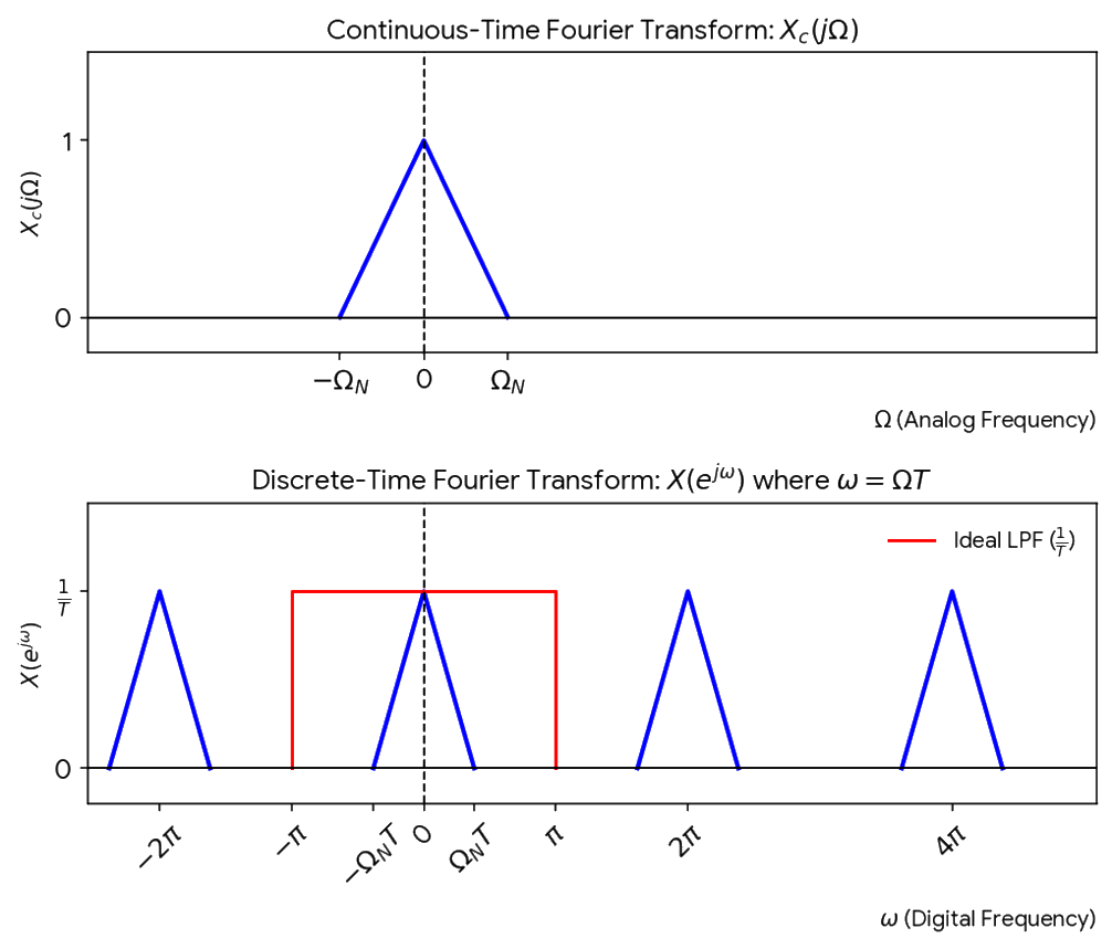
In other words, the frequency response of the discrete time sampled signal \(X_d(e^{j \Omega})\) maintains the same profile as the original continuous time sampled signal with some frequency and amplitude scaling and with periodic repetition in the \(\Omega\) domain.
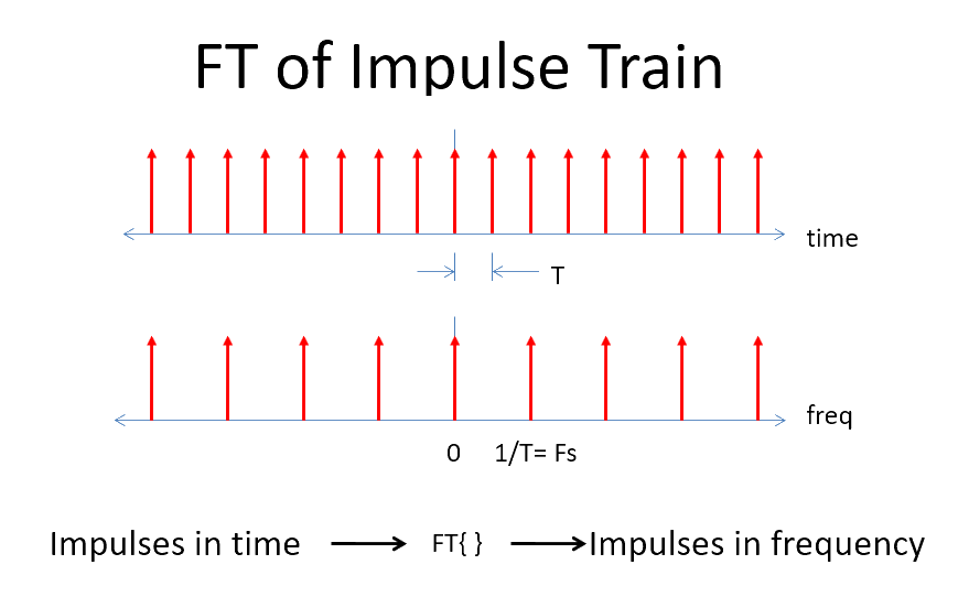
To determine the periodicity of the frequency response, recall that in order to be periodic, the function must satisfy
\[
\begin{align}
\forall \Omega, \exists \Omega_0:&& X_d(e^{j \Omega}) &= X_d(e^{j(\Omega + \Omega_0)}) \\
&&\frac{1}{T} \sum_{k=-\infty}^{\infty} X_c\left( j \frac{\Omega – 2 \pi k}{T}\right) &= \frac{1}{T} \sum_{l=-\infty}^{\infty} X_c\left( j \frac{(\Omega + \Omega_0) – 2 \pi l}{T}\right) \\
&&\frac{\Omega – 2 \pi k}{T} &= \frac{(\Omega + \Omega_0) – 2 \pi l}{T} \\
&&\Omega – 2 \pi k &= \Omega + \Omega_0 – 2 \pi l \\
&&\Omega_0 &= 2 \pi (l – k)
\end{align}
\]
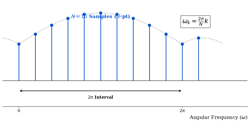
Because \(l,k \in \mathbb{Z}\), the period in the \(\Omega\) domain is \(2 \pi\). This matches our expectations for discrete signals. In summary, sampling a signal in the continuous time and representing it in discrete time is represented by the transform
\[
\begin{align}
x_d[n] = x_c(nT) &\stackrel{\mathcal{F}}{\leftrightarrow}
X_d(e^{j \Omega}) = \frac{1}{T} \sum_{k=-\infty}^{\infty} X_c\left( j \frac{\Omega – 2 \pi k}{T}\right) \\
\end{align}
\]
Impulse Invariance: Continuous to Discrete Time System Equivalence
If the impulse response of a continuous time system is sampled, the discrete impulse response is represented by
\[
\begin{align}
h_d[n] = h_c(nT) &\stackrel{\mathcal{F}}{\leftrightarrow} H_d(e^{j \Omega}) = \frac{1}{T} \sum_{k=-\infty}^{\infty} H_c\left( j \frac{\Omega – 2 \pi k}{T}\right) \\
\end{align}
\]
so that the system output is
\[
\begin{align}
y_d[n] &\stackrel{\mathcal{F}}{\leftrightarrow} Y_d(e^{j \Omega}) = H_d (e^{j \Omega}) X_d(e^{j \Omega}) \\
y_d[n] &\stackrel{\mathcal{F}}{\leftrightarrow} Y_d(e^{j \Omega}) = H_d (e^{j \Omega}) \left[ \frac{1}{T} \sum_{k=-\infty}^{\infty} X_c\left( j \frac{\Omega – 2 \pi k}{T}\right) \right] \\
y_d[n] &\stackrel{\mathcal{F}}{\leftrightarrow} Y_d(e^{j \Omega}) = \frac{1}{T} \sum_{k=-\infty}^{\infty} H_d (e^{j \Omega}) X_c\left( j \frac{\Omega – 2 \pi k}{T}\right) \\
\end{align}
\]
Note that if we were to scale the sampled impulse response by \(T\) to generate a new discrete system \(h[n]\), we would have
\[
\begin{align}
h[n] = T h_d[n] = T h_c(nT) &\stackrel{\mathcal{F}}{\leftrightarrow} H(e^{j \Omega}) = T H_d(e^{j \Omega}) = \sum_{k=-\infty}^{\infty} H_c\left( j \frac{\Omega – 2 \pi k}{T}\right) \\
\end{align}
\]
which eliminates the scaling factor in the discrete output
\[
\begin{align}
y_d[n] &\stackrel{\mathcal{F}}{\leftrightarrow} Y_d(e^{j \Omega}) = H (e^{j \Omega}) X_d(e^{j \Omega}) \\
y_d[n] &\stackrel{\mathcal{F}}{\leftrightarrow} Y_d(e^{j \Omega}) = \frac{1}{T} \sum_{k=-\infty}^{\infty} H (e^{j \Omega}) X_c\left( j \frac{\Omega – 2 \pi k}{T}\right) \\
y_d[n] &\stackrel{\mathcal{F}}{\leftrightarrow} Y_d(e^{j \Omega}) = \frac{1}{T} \sum_{k=-\infty}^{\infty} T H_d (e^{j \Omega}) X_c\left( j \frac{\Omega – 2 \pi k}{T}\right) \\
y_d[n] &\stackrel{\mathcal{F}}{\leftrightarrow} Y_d(e^{j \Omega}) = \sum_{k=-\infty}^{\infty} H_d (e^{j \Omega}) X_c\left( j \frac{\Omega – 2 \pi k}{T}\right) \\
\end{align}
\]
Assuming we are only concerned with \(|\Omega| < \pi \implies k = 0\)
\[
\begin{align}
y_d[n] &\stackrel{\mathcal{F}}{\leftrightarrow} Y_d(e^{j \Omega}) = H_d (e^{j \Omega}) X_c \left( j \frac{\Omega}{T}\right) \\
\end{align}
\]
which appears very similar to the LTI output (convolving impulse response leads to pure multiplication in the frequency domain).
The method of scaling the impulse response to emulate a desired continuous time filter is known as impulse invariance. In other words, when
\[
\begin{align}
h[n] = T h_c(nT)
\end{align}
\]
then \(h[n]\) is said to be an impulse invariant version of \(h_c(t)\).
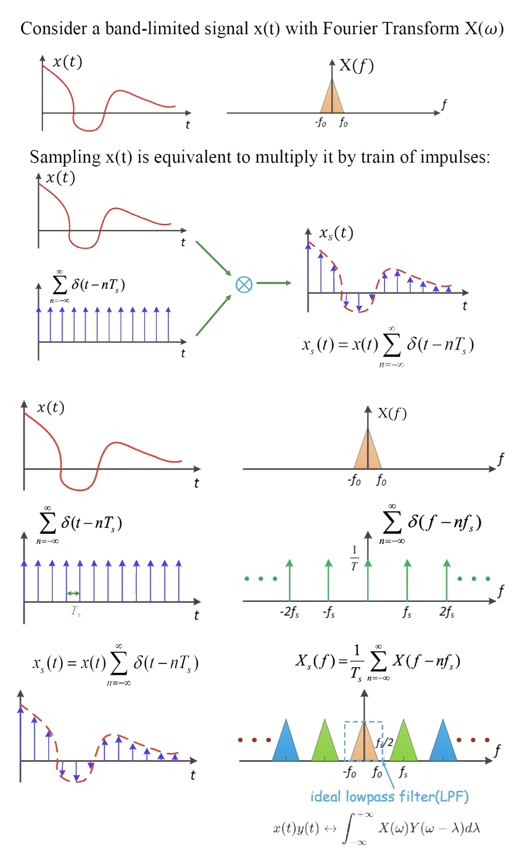
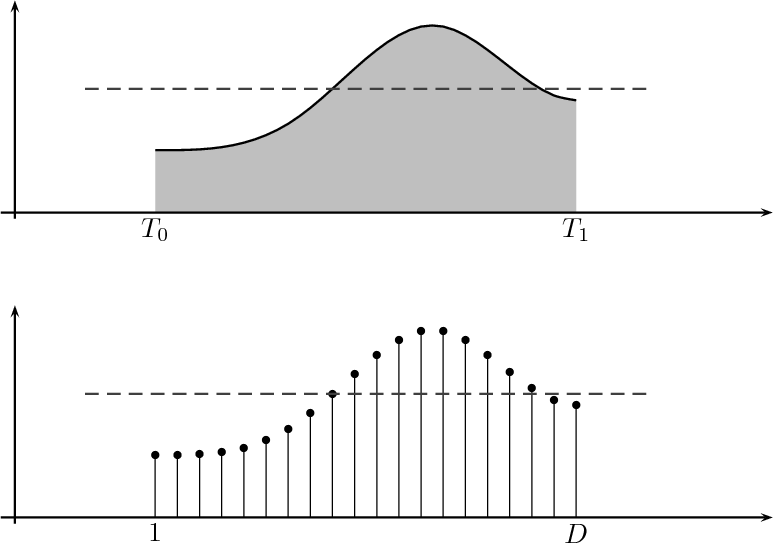
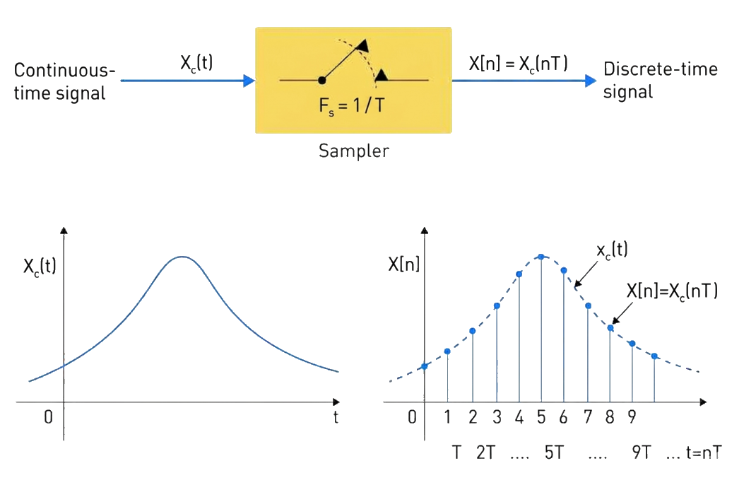
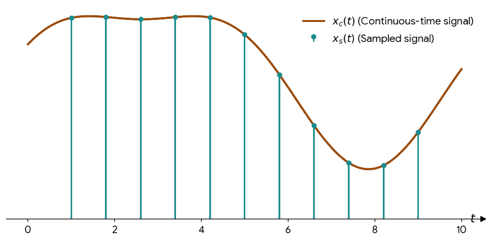
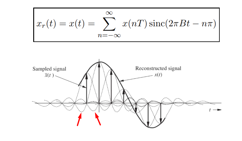
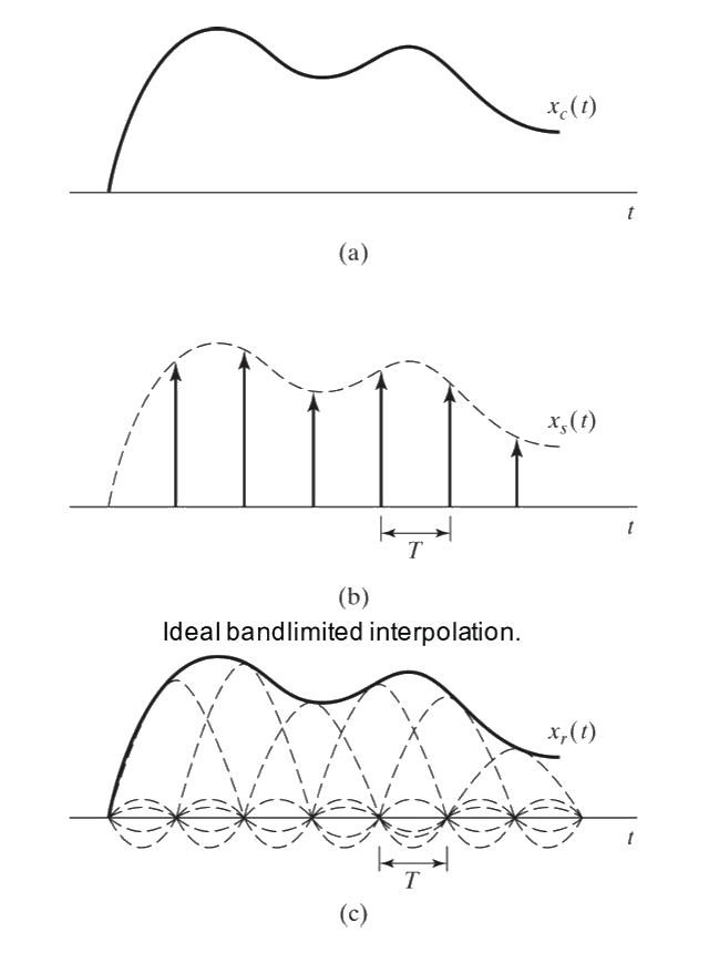
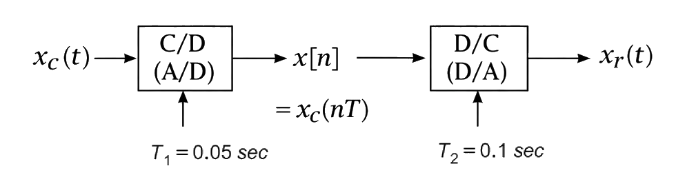
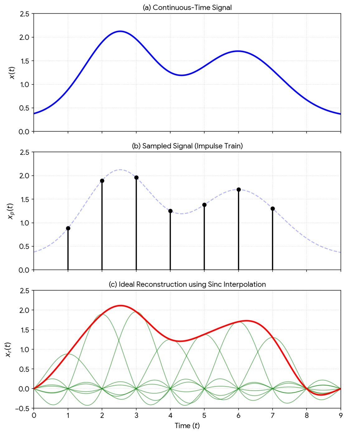
Signal Recovery
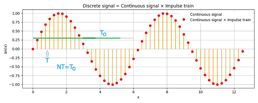
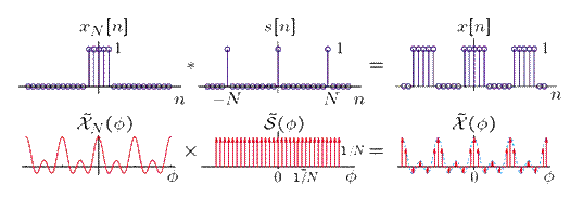
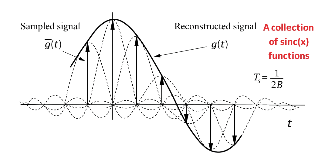
The process described for sampling a signal is effectively reversed when going from discrete to continuous time, and we first focus on generating an idealized continuous time sampled signal (weighted pulses spaced by \(T\)) from the discrete time sampled signal (sequence in \(n\)). The continuous time sampled signal then can be fed through continuous time Low pass filters (LPF) that represent various real-world interpolation methods to generate the re-created signal.
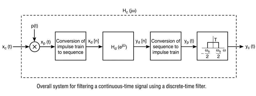
Discrete to Continuous Conversion

The impulse train can then be recreated for each discrete sample. That is
\[
\begin{align}
y_p(t) = \sum_{n=-\infty}^{\infty} y_d[n] \delta(t-nT)
&\stackrel{\mathcal{F}}{\leftrightarrow}
Y_p(j \omega) = \sum_{n=-\infty}^{\infty} y_d[n] e^{-j \omega n T} \\
\end{align}
\]
The discrete sample signal frequency response \(Y_d\) will repeat every \(2\pi\) in the \(\Omega\) domain as any discrete signal would. We also know that the output continuous signal frequency response \(Y_p(j \omega)\) will repeat in the \(\omega\) domain relative to the output sampling frequency \(\omega_s = 2 \pi / T\), and so \(\Omega = \omega T\) still holds as a viable comparison between \(\Omega\) and \(\omega\) domains.
This pulsed output signal \(Y_p(j \omega)\) contains information of the single desired result we want in the continuous domain, which we can denote as the idealized \(Y_c\) which is repeated every \(\omega_s\) in the \(\omega\) domain and scaled.
\[
\begin{align}
Y_p(j \omega) &= \frac{1}{T} \sum_{k=-\infty}^{\infty} Y_c(j(\omega – k \omega_s)) \\
\end{align}
\]
From this, we can see that to accurately recreate \(Y_d\) in continuous time, the ideal filter applied to \(Y_p\) scales all signals \(0 < |\omega| < \omega_s / 2\) by \(T\), and all other frequency information is removed. This idealized interpolation method is explored further below.
Note that the following discussion reverts back to using signal \(x\) instead of signal \(y\) for generality.
Interpolation
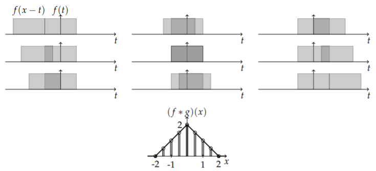
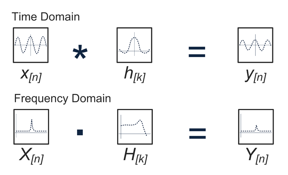
An interpolation formula describes how to fit a continuous curve between sample points \(x(nT)\) using a filter \(h(t)\mathop{\leftrightarrow}\limits^{{\mathcal{F}}}H(j\omega )\). Note that the shape of the filter impulse response \(h(t)\) is convolved with the idealized continuous sample pulse \(x_p(t)\) to represent the recovered signal.
\[
\begin{align}
x_r(t) &= x_p(t) * h(t) \\
x_r(t) &= \left[ \sum_{n=-\infty}^{\infty} x(nT) \delta(t-nT) \right] * h(t) \\
x_r(t) &= \sum_{n=-\infty}^{\infty} x(nT) h(t – nT) \\
\\
X_r(j \omega) &= X_p(j \omega) H(j \omega) \\
\end{align}
\]
The analysis does not need to be limited to the idealized continuous time sampled signal, and the same result appears if using discrete sampled values and the discrete frequency response.
\[
\begin{align}
x_r(t) &= \sum_{n=-\infty}^{\infty} x_d[n] * h(t – nT) \\
\\
X_r(j \omega) &= \sum_{n=-\infty}^{\infty} x_d[n] H(j \omega) e^{-j \omega T n} \\
X_r(j \omega) &= H(j \omega) \sum_{n=-\infty}^{\infty} x_d[n] e^{-j \omega T n} \\
X_r(j \omega) &= H(j \omega) \sum_{n=-\infty}^{\infty} x_d[n] e^{-j \Omega n} \\
X_r(j \omega) &= H(j \omega) X_d(e^{j \Omega}) \\
\end{align}
\]
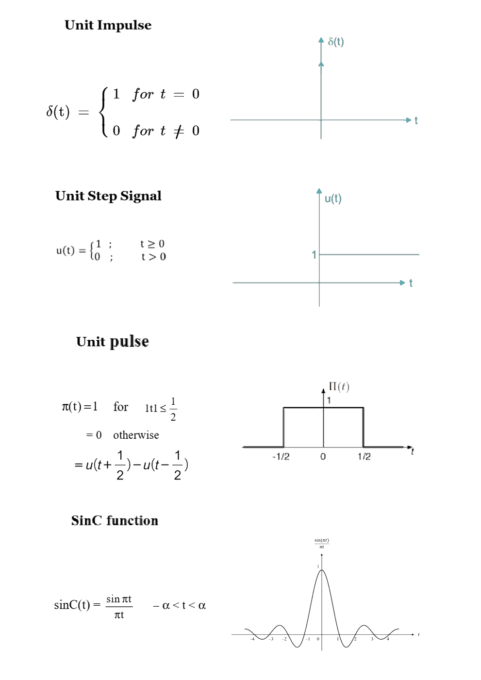
Ideal Signal Recreation Filter / Ideal Low-Pass Filter
This filter recreates the original signal perfectly such that \(x_r(t) = x(t)\) It is difficult to implement in real-life, but provides a useful foundation of analysis.
A unity-gain low-pass filter is described by
\[H_u(j\omega)=\left\{\begin{array}{lc}1&\left|\omega\right|<\omega_c\\0&\left|\omega\right|\geq\omega_c\end{array}\right.\]
Which can be found to have a frequency response of
\[
\begin{align}
h_u(t) &= \frac{\sin(\omega_c t)}{\pi t} \\
\end{align}
\]
Recall that the magnitude of \(X_p(j \omega)\) is \(X(j \omega)\) scaled by \(1/T\), so in order to get the recovered signal spectrum \(X_r(j \omega)\), we would need to scale the filter by the sampling period, \(T\). That is, the ideal signal recovery interpolation filter is described by
\[H(j\omega)=\left\{\begin{array}{lc}T&\left|\omega\right|<\omega_c\\0&\left|\omega\right|\geq\omega_c\end{array}\right.\]
\[
\begin{align}
H(j \omega) = T H_u (j \omega)
\end{align}
\]
\[
\begin{align}
h(t) &= T \frac{\sin(\omega_c t)}{\pi t} \\
h(t) &= \frac{\omega_c T}{\pi} \frac{\sin(\omega_c t)}{\omega_c t} \\
h(t) &= \frac{\omega_c T}{\pi} sinc(\omega_c t) \\
\end{align}
\]
So the recovered signal becomes
\[
\begin{align}
x_r(t) &= \sum_{n=-\infty}^{\infty} x(nT) \frac{\omega_c T}{\pi} \frac{\sin(\omega_c (t-nT))}{\omega_c (t-nT)} \\
\end{align}
\]
In the case where we assume the signal is band-limited and no aliasing occurs, we can use \(\omega_c = \omega_s/2 = \pi/T\) to get
\[
\begin{align}
h(t) &= \frac{\sin(\pi t / T)}{\pi t / T} \\
h(t) &= sinc(\pi t / T) \\
\end{align}
\]
The reconstructed signal is then described by
\[
\begin{align}
x_r(t) &= \sum_{n=-\infty}^{\infty} x(nT) h(t – nT) \\
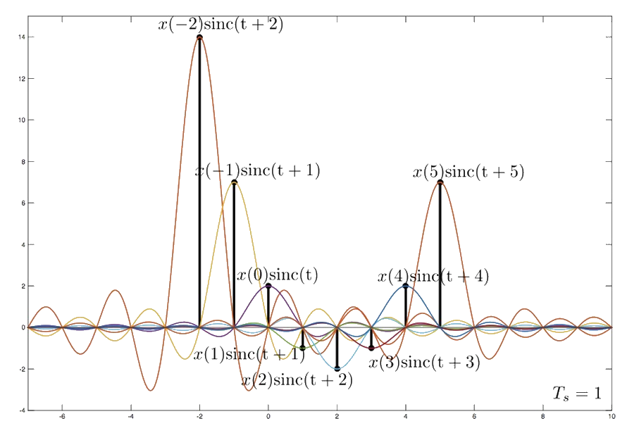
x_r(t) &= \sum_{n=-\infty}^{\infty} x(nT) \frac{\sin[\pi (t – nT) / T]}{\pi (t – nT) / T} \\
x_r(t) &= \sum_{n=-\infty}^{\infty} x[n] \frac{\sin[\pi (t – nT) / T]}{\pi (t – nT) / T} \\
\end{align}
\]
In other words, the summation of sinc functions at each time step scaled by the original signal exactly replicates the original signal.
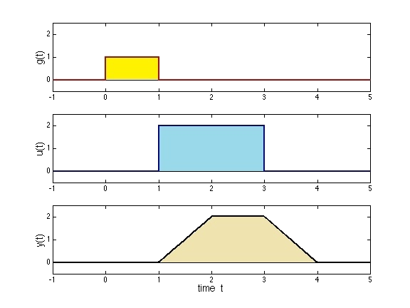
Zero-Order Hold (ZOH)
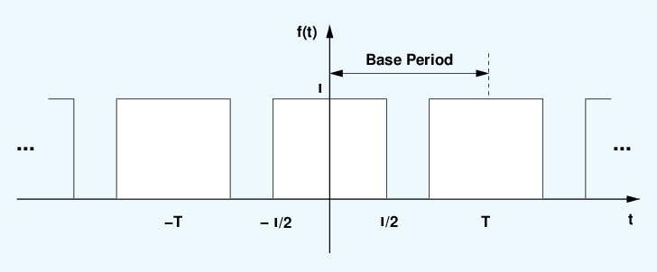
More common in practice than multiplying input signal by generated impulses. Output is equivalent to convolving \(x_p(t)\) (same as above) with a filter, \(H_0(j \omega)\), that has impulse response, \(h_0(t)\), that is unity between \(t=0\) and \(t=T\).
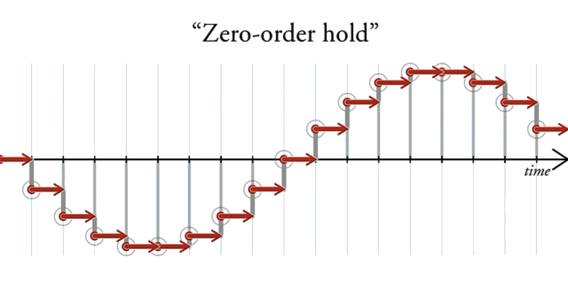
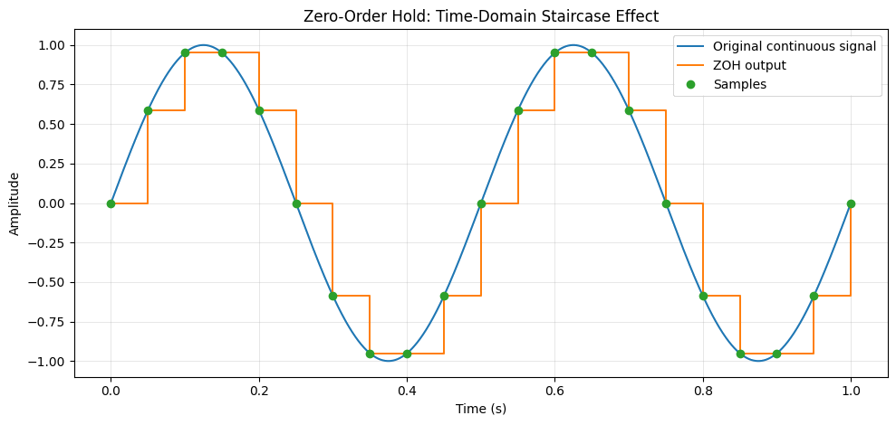
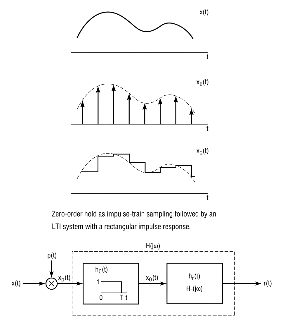
Note that \(H_0(j \omega)\) is very similar to the rectangular pulse, but shifted in time.
\[
\begin{align}
H_{sq} (j \omega) &= \frac{2 sin(\omega T/2)}{\omega}
&& \text{Square of width }T\text{, centered at }t=0 \\
H_0 (j \omega) &= e^{-j \omega T/2} \frac{2 sin(\omega T/2)}{\omega}
&& \text{Square of width }T\text{, delayed by }t=T/2 \\
\end{align}
\]
If the effects of the Zero-Order hold are desired to be reversed, an ideal reconstruction filter \(H_r(j \omega)\) would be
\[
\begin{align}
H_0(j \omega) H_r(j \omega) &= 1 \\
H_r(j \omega) &= \frac{1}{H_0(j \omega)} \\
H_r(j \omega) &= \frac{1}{e^{-j \omega T/2} \frac{2 sin(\omega T/2)}{\omega}} \\
H_r(j \omega) &= \frac{e^{j \omega T/2}}{\frac{2 sin(\omega T/2)}{\omega}} \\
\end{align}
\]
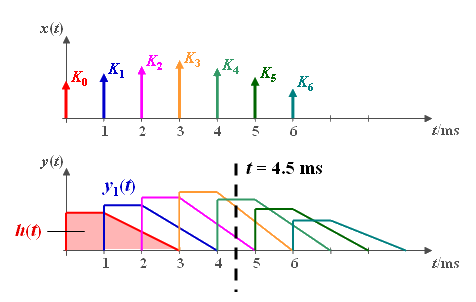
First-Order Hold/Linear Interpolation
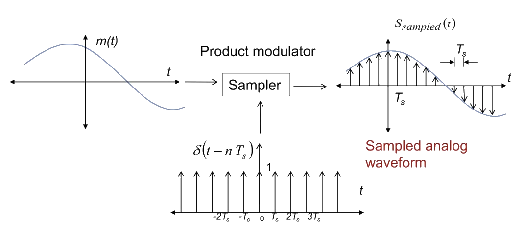
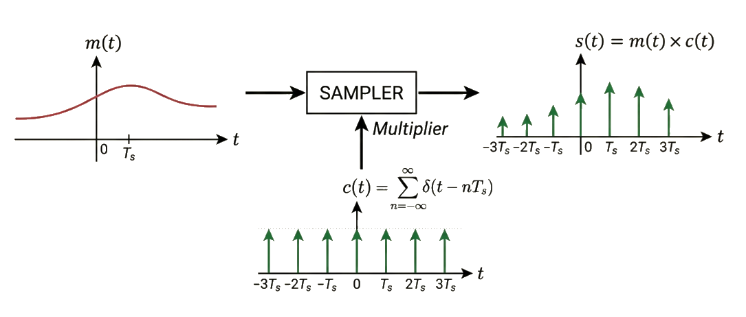
Consider \(x_p(t)\), the series of impulses weighted by \(x(t)\)
\[
\begin{align}
x_p(t) &= \sum_{n=-\infty}^{\infty} x(nT) \delta(t-nT) \\
\end{align}
\]
An interpolating filter \(h(t)\) would then generate a recreated signal, \(x_r(t)\) be described as
\[
\begin{align}
x_r(t) &= x_p(t) * h(t) \\
x_r(t) &= \left[ \sum_{n=-\infty}^{\infty} x(nT) \delta(t-nT) \right] * h(t) \\
x_r(t) &= [ \cdots + x(-2T)\delta(t+2T) + x(-T)\delta(t+T) + x(0)\delta(t) + \\
&x(T)\delta(t-T) + x(2T)\delta(t-2T) + \cdots] * h(t) \\
x_r(t) &= \cdots + x(-2T)h(t+2T) + x(-T)h(t+T) + x(0)h(t) + \\
&x(T)h(t-T) + x(2T)h(t-2T) + \cdots \\
\end{align}
\]
Alternatively, one can find more simply that
\[
\begin{align}
x_r(t) &= x_p(t) * h(t) \\
x_r(t) &= \left[ \sum_{n=-\infty}^{\infty} x(nT) \delta(t-nT) \right] * h(t) \\
x_r(t) &= \sum_{n=-\infty}^{\infty} x(nT) \left[ \delta(t-nT) * h(t) \right] \\
x_r(t) &= \sum_{n=-\infty}^{\infty} x(nT) h(t-nT) \\
\end{align}
\]
If we confine our focus to the region between two impulses of \(x_p(t)\), say at some \(t_0\), we can make some conceptual simplifications to determine the interpolation function. Note that in this case, all impulses of \(x_p(t)\) where \(t > t_0\) are weighted by the acausal side of \(h(t)\) (\(t < 0\)) whereas all the impulses of \(x_p(t)\) where \(t \leq t_0\) are weighted by the causal half of \(h(t)\) (\(t \geq 0\)). Graphically, we can split \(h(t)\) into two functions where
\[ h(t) = h_{pre}(t) + h_{post}(t) \]

Now with knowledge of what we want as the output, we can define the interpolation function. For example if we know that we want
\[
\begin{align}
x_r(t_0) = x(t_0) && { t_0 | t_0=nT, n \in \mathbb{Z}} \\
\end{align}
\]
then
\[
\begin{align}
x_r(0) &= \cdots + x(-2T)h(2T) + x(-T)h(T) + x(0)h(0) + \\
&x(T)h(-T) + x(2T)h(-2T) + \cdots \\
\\
&= x(0)\\
\end{align}
\]
and
\[
\begin{align}
x_r(T) &= \cdots + x(-2T)h(T+2T) + x(-T)h(T+T) + x(0)h(T) + \\
&x(T)h(T-T) + x(2T)h(T-2T) + \cdots \\
&= \cdots + x(-2T)h(3T) + x(-T)h(2T) + x(0)h(T) + \\
&x(T)h(0) + x(2T)h(-T) + \cdots \\
&= x(T)\\
\end{align}
\]
then to be agnostic of the input function, \(x(t)\), we must set
\[
\begin{align}
h(0) = 1 \\
h(t) = 0 && \forall |t| \geq T
\end{align}
\]
Now, let’s pick \(t_0 \in [0,T]\) and only look at this interval. In this case we can rewrite \(x_r(t)\) as
\[
\begin{align}
x_r(t_0) &= \cdots + x(-2T)h_{post}(t_0+2T) + x(-T)h_{post}(t_0+T) + x(0)h_{post}(t_0) + \\
&x(T)h_{pre}(t_0-T) + x(2T)h_{pre}(t_0-2T) + \cdots && t_0 \in [0,T] \\
\end{align}
\]
Applying these constraints, \(x_r(t)\) has many terms that become 0 and it simplifies to
\[
\begin{align}
x_r(t_0) &= x(0)h_{post}(t_0) + x(T)h_{pre}(t_0-T) && t_0 \in [0,T] \\
\end{align}
\]
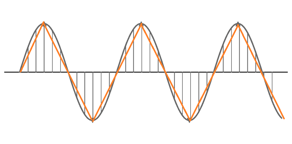
Additionally, if we want \(x_r(t_0)\) to resemble a line between the two samples (first-order hold/linear interpolation), we set the equation of that line equal to \(x_r(t)\) then solve for the impulse response function that makes that possible.
\[
\begin{align}
x(0)h_{post}(t_0) + x(T)h_{pre}(t_0-T) &= x(0) + \frac{x(T) – x(0)}{T} t_0 && t_0 \in [0,T] \\
x(0)h_{post}(t_0) + x(T)h_{pre}(t_0-T) &= x(0) + \frac{1}{T} x(T) t_0 – \frac{1}{T}x(0) t_0 && t_0 \in [0,T] \\
x(0)h_{post}(t_0) + x(T)h_{pre}(t_0-T) &= x(0)\left[1 – \frac{t_0}{T} \right] + x(T) \frac{t_0}{T} && t_0 \in [0,T] \\
\end{align}
\]
The impulse response function can then be isolated such that
\[
\begin{align}
h_{post}(t) = 1 – \frac{t}{T} \\
h_{post}(t) = \frac{T – t}{T} \\
\\
h_{pre}(t-T) = \frac{t}{T} \\
h_{pre}(t) = \frac{t+T}{T} \\
\end{align}
\]
and so the final impulse response is
\[h(t)=\left\{\begin{array}{lc}\frac{t+T}T&-T<t<0\\\frac{T-t}T&0\leq t<T\\0&otherwise\end{array}\right.\]
Note that the impulse response is acausal, but \(h(t) = 0 \;\;\; \forall t > T\), so one can effectively achieve linear interpolation with a latency of \(T\).
Transfer function is determined by taking derivatives
\[h'(t)=\left\{\begin{array}{lc}\frac1T&-T<t<0\\\frac{-1}T&0\leq t<T\\0&otherwise\end{array}\right.\]
\[
h”(t) = \frac{1}{T} \delta(t+T) – \frac{2}{T} \delta(t) + \frac{1}{T} \delta(t-T)
\]
\[
\begin{align}
H”(j \omega) = \frac{1}{T} e^{j \omega T} – \frac{2}{T} + \frac{1}{T} e^{-j \omega T} \\
H”(j \omega) = \frac{1}{T} \left[ e^{j \omega T} + e^{-j \omega T} -2 \right] \\
\end{align}
\]
\[
\begin{align}
H(j \omega) = \frac{1}{(j \omega)^2 T} \left[2 \cos(\omega T) -2 \right] &&\omega \neq 0 \\
H(j \omega) = \frac{2}{(j \omega)^2 T} \left[\cos(\omega T) – 1 \right] &&\omega \neq 0 \\
\end{align}
\]
Half Angle Formula
\[
\begin{array}{ll}
sin^2(x) = \frac{1 – cos(2x)}{2} \\
2 sin^2(x) = 1 – cos(2x) \\
cos(2x) – 1 = – 2 sin^2(x)
\end{array}
\]
\[
\begin{align}
2x = \omega T \\
x = \frac{\omega T}{2} \\
\end{align}
\]
\[
\begin{align}
H(j \omega) = \frac{2}{(j \omega)^2 T} \left[ -2 \sin^2 \left( \frac{\omega T}{2} \right) \right] &&\omega \neq 0 \\
H(j \omega) = \frac{-4 \sin^2 (\omega T/2)}{(j \omega)^2 T} &&\omega \neq 0 \\
H(j \omega) = \frac{1}{T} \frac{4 \sin^2 (\omega T/2)}{ \omega^2} &&\omega \neq 0 \\
H(j \omega) = \frac{1}{T} \frac{\sin^2 (\omega T/2)}{ (\omega / 2)^2} &&\omega \neq 0 \\
H(j \omega) = T \frac{\sin^2 (\omega T/2)}{ (\omega T / 2)^2} &&\omega \neq 0 \\
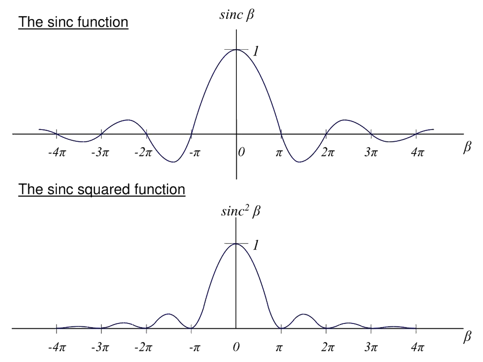
H(j \omega) = T sinc^2 (\omega T/2) &&\omega \neq 0 \\
H(j \omega) = \frac{2 \pi}{\omega_s} sinc^2 \left(\pi \frac{\omega}{\omega_s} \right) &&\omega \neq 0 \\
\end{align}
\]