


Mathematics Yoshio Jul 28th, 2025 at 8:00 PM 8 0
Z-transform
\(\begin{array}{cc}DTFT&\\X(e^{j\omega})=\sum_{n=-\infty}^\infty x\lbrack n\rbrack e^{-j\omega n}&\Leftrightarrow\end{array}\begin{array}{c}Z-transform\\X(z)=\sum_{n=-\infty}^\infty x\lbrack n\rbrack e^{-z}\end{array}\)
\(z\) is a complex number (real part and imaginary part)
\(e^{j\omega}\) is only imaginary part. DTFT is a special case in Z-transform, \(z=e^{j\omega}\)
DTFT is used for signals, Z-transform is used for system
Discrete-time Fourier transform
\(X(e^{j\omega})={\textstyle\sum_{n=-\infty}^\infty}x\lbrack n\rbrack e^{-j\omega n}\)
\(x\lbrack n\rbrack=\frac1{2\pi}\int_{-\pi}^\pi{X(e^{j\omega})}e^{j\omega n}\operatorname d\omega\)
\(x\lbrack n\rbrack=a^nu\lbrack n\rbrack\;\xrightarrow{DTFT}X(e^{j\omega})=\sum_{n=0}^\infty a^ne^{-j\omega n}=\frac1{1-ae^{-j\omega}},\;\left|a\right|<1\)
\(x\lbrack n\rbrack=5^nu\lbrack n\rbrack\nrightarrow X(e^{j\omega})\)
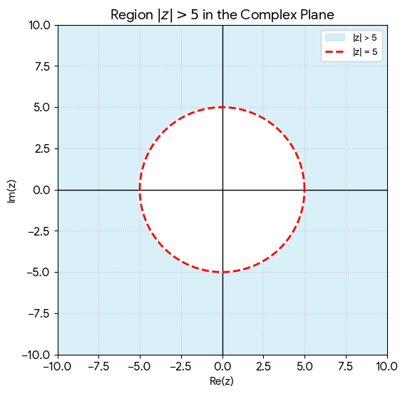
\(x\lbrack n\rbrack=5^nu\lbrack n\rbrack\overset{\mathcal Z}\leftrightarrow X(z)=\frac1{1-5z^{-1}},\;\left|5z^{-1}\right|<1,\;\left|z\right|>5\)
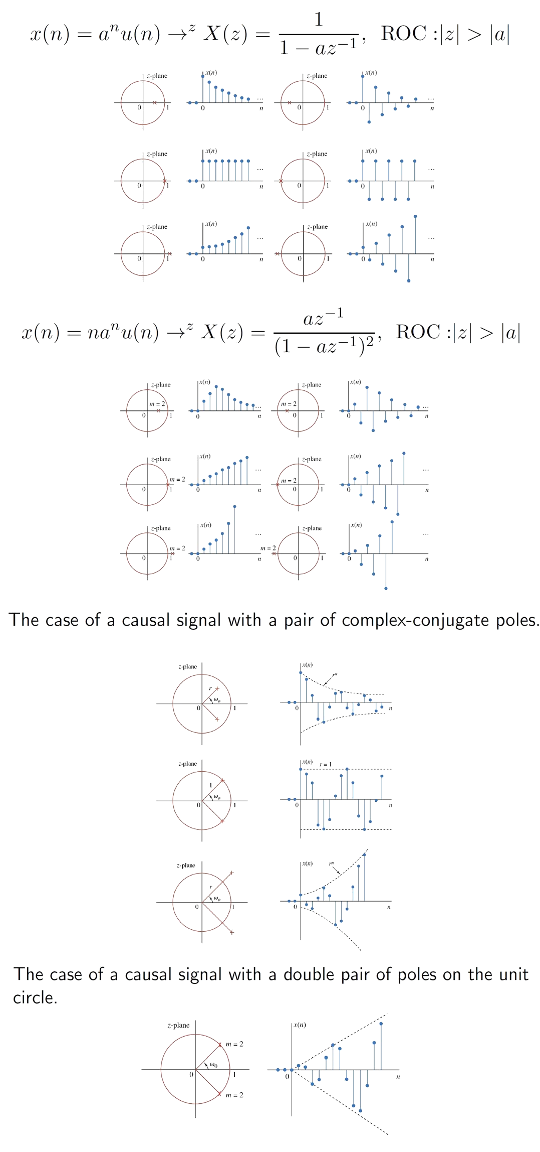
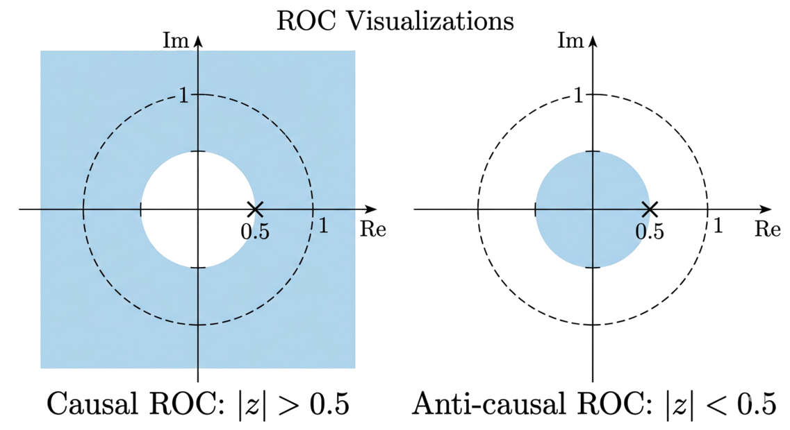
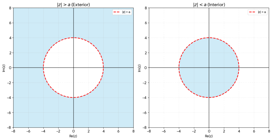
[A] \(x\lbrack n\rbrack=a^nu\lbrack n\rbrack\overset{\mathcal Z}\leftrightarrow X(z)=\frac1{1-az^{-1}},\;\left|az^{-1}\right|<1,\;\left|z\right|>\left|a\right|\)
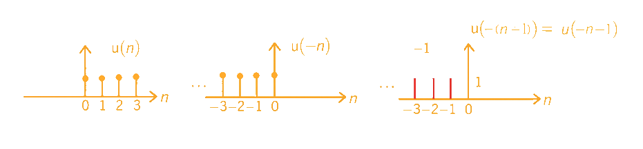
[B] \(x\lbrack n\rbrack=-a^nu\lbrack-n-1\rbrack\)
\(X(z)=\sum_{n=-\infty}^\infty-a^nu\lbrack-n-1\rbrack z^{-n}\\x\lbrack n\rbrack=-a^nu\lbrack-n-1\rbrack\)
\(=\sum_{n=-\infty}^{-1}-a^nz^{-n}\), Let \(m=-n\)
\(=\sum_{m=1}^\infty-{(a^{-1}z)}^m\)
\(=\sum_{m=0}^\infty-{(a^{-1}z)}^m+1\)
\(=1-\frac1{1-(a^{-1}z)},\;\left|a^{-1}z\right|<1\Rightarrow\left|z\right|<\left|a\right|\)
\(=\frac{1-a^{-1}z-1}{1-a^{-1}z}=\frac{-a^{-1}z}{1-a^{-1}z}=\frac1{1-az^{-1}}\)
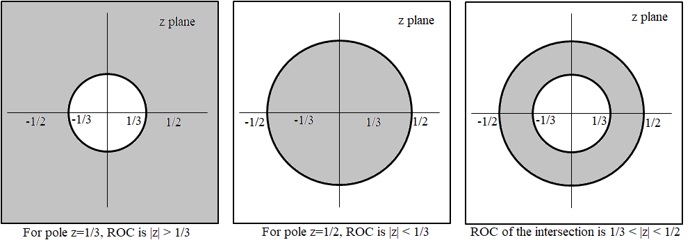
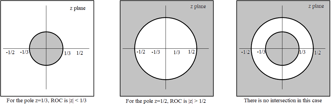
\(\left\{\begin{array}{lc}a^nu\lbrack n\rbrack\overset{\mathcal Z}\leftrightarrow\frac1{1-az^{-1}},\;\left|z\right|>\left|a\right|&right-sided\;sequence\\-a^nu\lbrack-n-1\rbrack\overset{\mathcal Z}\leftrightarrow\frac1{1-az^{-1}},\;\left|z\right|<\left|a\right|&left-sided\;sequence\end{array}\right.\)
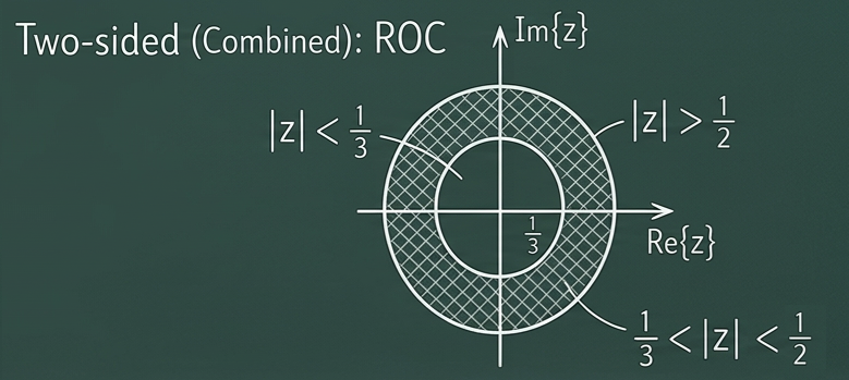
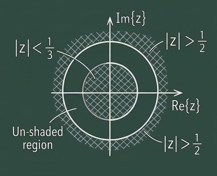
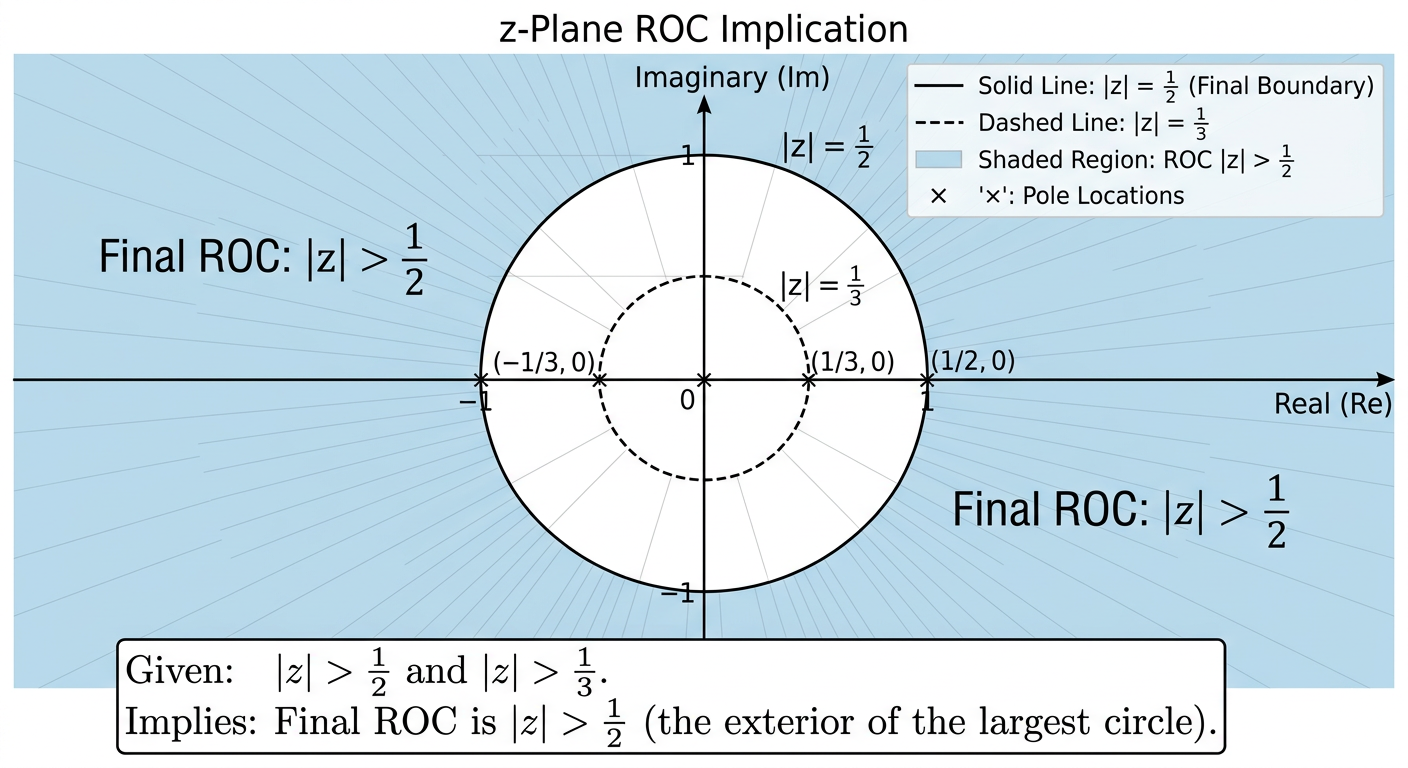
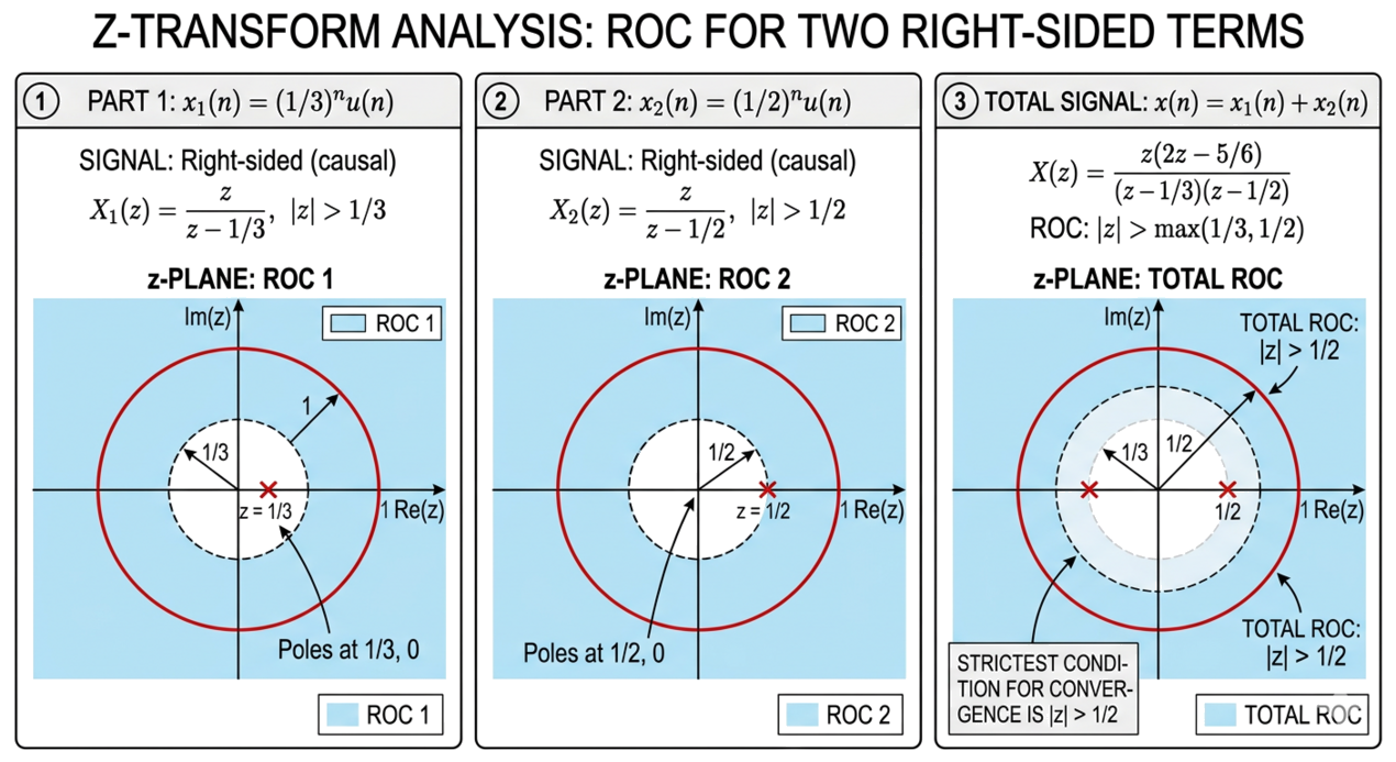
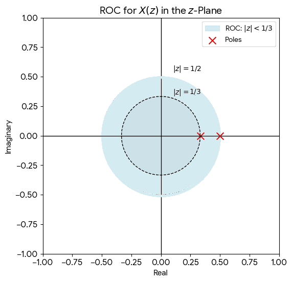
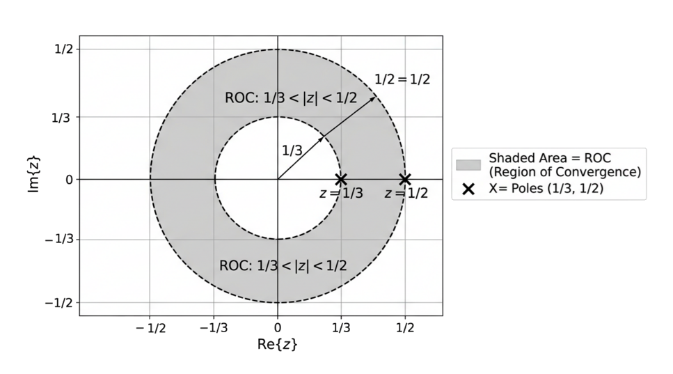
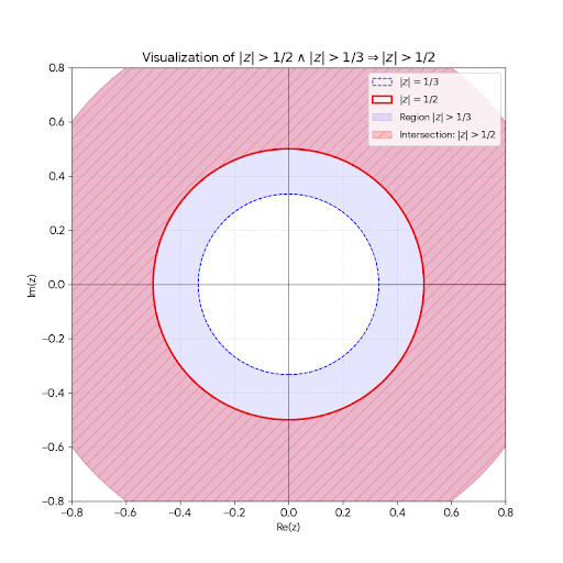
[Ex] \(x\lbrack n\rbrack={(\frac12)}^nu\lbrack n\rbrack+{(-\frac13)}^nu\lbrack n\rbrack\)
\(X(z)=\frac1{1-{\frac12}z^{-1}}+\frac1{1+{\frac13}z^{-1}}\)
\(\left|z\right|>\frac12\;\&\;\left|z\right|>\frac13\;\Rightarrow\;\left|z\right|>\frac12\)
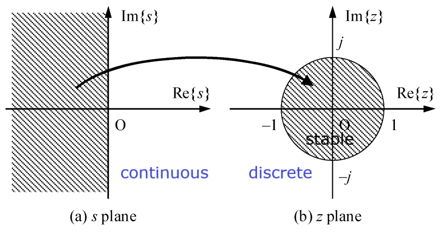
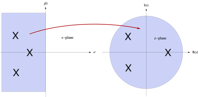
In mathematics and signal processing, the Z-transform converts a discrete-time signal, which is a sequence of real or complex numbers, into a complex valued frequency-domain (the z-domain or z-plane) representation.
It can be considered a discrete-time equivalent of the Laplace transform (the s-domain or s-plane). This similarity is explored in the theory of time-scale calculus.
Discretized system and Z-transform
\(u(t)\rightarrow H(s)\rightarrow y(t)\)
\(\left\{\begin{array}{l}\underline{\dot x}(t)=A\underline x(t)+\underline bu(t)\\y(t)=\underline c\underline x(t)\end{array}\right.\)
\(\underline x(t)=e^{\underline At}{\underline x}_0+\int_0^te^{{\underline A(t-\tau)}}\underline bu(\tau)\operatorname d\tau\)
\(t=kT\)
\(\underline x(kT)=e^{\underline AkT}{\underline x}_0+\int_0^{kT}e^{{\underline A(kT-\tau)}}\underline bu(\tau)\operatorname d\tau\)
\(\underline x((k+1)T)=e^{\underline A(k+1)T}{\underline x}_0+\int_0^{(k+1)T}e^{{\underline A((k+1)T-\tau)}}\underline bu(\tau)\operatorname d\tau\)
\(=e^{\underline AT}(e^{\underline AkT}{\underline x}_0+\int_0^{(k+1)T}e^{{\underline A(kT-\tau)}}\underline bu(\tau)\operatorname d\tau)\)
\(=e^{\underline AT}(\underline x(kT)+\int_{kT}^{(k+1)T}e^{{\underline A(kT-\tau)}}\underline bu(\tau)\operatorname d\tau)\)
\(=e^{\underline AT}\underline x(kT)+\int_{kT}^{(k+1)T}e^{{\underline A((k+1)T-\tau)}}\underline bu(\tau)\operatorname d\tau)\)
\(\left\{\begin{array}{l}\underline x(kT)=e^{\underline AkT}{\underline x}_0+\int_0^{kT}e^{{\underline A(kT-\tau)}}\underline bu(\tau)\operatorname d\tau\\\underline x((k+1)T)=e^{\underline AT}\underline x(kT)+\int_{kT}^{(k+1)T}e^{{\underline A((k+1)T-\tau)}}\underline bu(\tau)\operatorname d\tau)\end{array}\right.\)
Let \(u(t)=u(kT)\;for\;kT\leq t<(k+1)T\)
\(\underline x(kT)=\underline x\lbrack k\rbrack,\;u(kT)=u\lbrack k\rbrack\)
then \(\underline x\lbrack k+1\rbrack=e^{\underline AT}\underline x\lbrack k\rbrack+(\int_{kT}^{(k+1)T}e^{{\underline A((k+1)T-\tau)}}\underline b\operatorname d\tau)u\lbrack k\rbrack\)
Let \(\alpha=\tau-kT\) then \(d\alpha=d\tau\)
\(\Rightarrow\underline x\lbrack k+1\rbrack=e^{\underline AT}\underline x\lbrack k\rbrack+(\int_0^Te^{{\underline A(T-\alpha)}}\underline b\operatorname d\tau)u\lbrack k\rbrack\)
\(\Rightarrow\underline x\lbrack k+1\rbrack={\underline A}_T\underline x\lbrack k\rbrack+{\underline b}_Tu\lbrack k\rbrack\)
where \({\underline A}_T=e^{\underline AT},\;{\underline b}_T=\int_0^Te^{{\underline A(T-\alpha)}}\underline b\operatorname d\tau\)
Similar to \(\left\{\begin{array}{l}\underline x\lbrack k+1\rbrack=\underline A\underline x\lbrack k\rbrack+\underline bu\lbrack k\rbrack\\y\lbrack k\rbrack=\underline c\underline x\lbrack k\rbrack+d\lbrack k\rbrack\end{array}\right.\)
A direct method to discretize the system is given as,
\(\underline{\dot x}(t)\approx\frac{\underline x\lbrack k+1\rbrack-\underline x\lbrack k\rbrack}T\)
\(\therefore\frac{\underline x\lbrack k+1\rbrack-\underline x\lbrack k\rbrack}T=\underline A\underline x\lbrack k\rbrack+\underline bu\lbrack k\rbrack\)
\(\Rightarrow\underline x\lbrack k+1\rbrack\approx(\underline I+T\underline A)\underline x\lbrack k\rbrack+T\underline bu\lbrack k\rbrack,\;where\;T\;is\;small\;enough\)
\(\therefore e^{{\underline AT}}\approx\underline I+T\underline A\)
\(\int_0^Te^{{\underline A(T-\alpha)}}\underline b\operatorname d\tau\approx T\underline b\)
Analysis of \(e^{{\underline AT}}\)
\((e^x)'=e^x\)
\(\left\{\begin{array}{l}e^x=1+x+\frac1{2!}x^2+\frac1{3!}x^3+\cdots\\e^{{\underline AT}}=\underline I+T\underline A+\cancel{\frac1{2!}{(T\underline A)}^2}+\cancel{\frac1{3!}{(T\underline A)}^3}+\cdots\end{array}\right.\)
\(\int_0^Te^{{\underline A(T-\alpha)}}\underline b\operatorname d\tau=\int_0^T\lbrack\underline I+(T-\alpha)\underline A+\frac1{2!}{(T-\alpha)}^2\underline A^2+\frac1{3!}{(T-\alpha)}^3\underline A^3+\cdots\rbrack\underline b\operatorname d\tau\)
\(=(T\underline I+\cancel{T^2}\dots+\cancel{T^k}+\dots)\underline b\)
\(\simeq T\underline b\)
Linear algebra : diagonized
MATLAB \(expm(\underline A)\)
For a physical system, \(\underline A\) is generally stable.
That means all the eigenvalues of \(\underline A\) are located in the left-half complex plane.
\(e^{\underline AT}\rightarrow?\;(eigenvalues)\)
\(e^{\underline AT}\approx\underline I+T\underline A\)
[Ex] \(\underline A=\begin{bmatrix}0&1\\-2&-3\end{bmatrix}\)
\(\left|\lambda\underline I-\underline A\right|=\begin{vmatrix}\lambda&-1\\2&\lambda+3\end{vmatrix}=\lambda^2+3\lambda+2\)
\(\left|\lambda\underline I-\underline A\right|=0\;\Rightarrow\;\lambda=-1,\;-2\) stable
\(\left\{\begin{array}{l}\underline A{\underline v}_1=-{\underline v}_1\\\underline A{\underline v}_2=-2{\underline v}_2\end{array}\Rightarrow\right.\underline A\underbrace{\begin{bmatrix}{\underline v}_1&{\underline v}_2\end{bmatrix}}_\underline V=\underbrace{\begin{bmatrix}{\underline v}_1&{\underline v}_2\end{bmatrix}}_\underline V\underbrace{\begin{bmatrix}-1&0\\0&-2\end{bmatrix}}_\underline\Lambda\)
\(\underline A=\underline V\underline\Lambda\underline V^{-1}\)
\(\underline A^n=\underline V\underline\Lambda^n\underline V^{-1}=\underline V\begin{bmatrix}{(-1)}^n&0\\0&{(-2)}^n\end{bmatrix}\underline V^{-1}\)
\(e^{\underline AT}=\sum_{k=0}^\infty\frac1{k!}{(T\underline A)}^k\)
\(=\sum_{k=0}^\infty\frac1{k!}T^k\underline V\underline\Lambda^k\underline V^{-1}\)
\(=\underline V(\sum_{k=0}^\infty\frac1{k!}T^k\underline\Lambda^k)\underline V^{-1}\)
\(=\underline V(\sum_{k=0}^\infty\frac1{k!}\begin{bmatrix}{(-1)}^kT^k&0\\0&{(-2)}^kT^k\end{bmatrix})\underline V^{-1}\)
\(=\underline V\begin{bmatrix}\sum_{k=0}^\infty\frac1{k!}{(-1)}^kT^k&0\\0&\sum_{k=0}^\infty\frac1{k!}{(-2)}^kT^k\end{bmatrix}\underline V^{-1}\)
\(=\underline V\begin{bmatrix}e^{-T}&0\\0&e^{-2T}\end{bmatrix}\underline V^{-1}\)
\(\left|\lambda\underline I-e^{\underline AT}\right|=\left|\lambda\underline I-\underline V\begin{bmatrix}e^{-T}&0\\0&e^{-2T}\end{bmatrix}\underline V^{-1}\right|\)
\(=\left|\underline V\lambda\underline I\underline V^{-1}-\underline V\begin{bmatrix}e^{-T}&0\\0&e^{-2T}\end{bmatrix}\underline V^{-1}\right|\)
\(=\left|\underline V(\lambda\underline I-\begin{bmatrix}e^{-T}&0\\0&e^{-2T}\end{bmatrix})\underline V^{-1}\right|\)
\(=\left|\underline V\right|\left|\lambda\underline I-\begin{bmatrix}e^{-T}&0\\0&e^{-2T}\end{bmatrix}\right|\left|\underline V^{-1}\right|\)
\(=\left|\lambda\underline I-\begin{bmatrix}e^{-T}&0\\0&e^{-2T}\end{bmatrix}\right|\)
\(e^{\underline AT}\) eigenvalues are \(e^{-T},\;e^{-2T}\)
where \(e^{-T}=1-T+\cancel{\frac1{2!}{(-T)}^2}+\cancel\cdots\approx1-T<1\)
\(e^{-2T}\approx1-2T<1\)
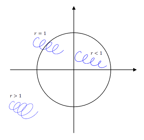
\(\underline A\;\rightarrow{\left.e^{\lambda t}\right|}_{t\rightarrow\infty}=0\)
\(e^{\underline AT}\rightarrow\left|\lambda\right|<1\)
\(\left\{\begin{array}{l}\underline x\lbrack k+1\rbrack=0.9\underline x\lbrack k\rbrack\rightarrow stable\\\underline x\lbrack k+1\rbrack=1.1\underline x\lbrack k\rbrack\rightarrow unstable\end{array}\right.\)
Consider a discretized system
\(\left\{\begin{array}{l}\underline x\lbrack k+1\rbrack=\underline A\underline x\lbrack k\rbrack+\underline bu\lbrack k\rbrack\\y\lbrack k\rbrack=\underline c\underline x\lbrack k\rbrack+\underbrace{\cancel{d\lbrack k}\rbrack}_{not\;considered}\end{array}\right.\)
difference equation = ?
\(\underline A\in R^{n\times n}\;eigenvalues\;\left|\lambda\right|<1\)
\(\left|\lambda\underline I-\underline A\right|=\lambda^n+a_{n-1}\lambda^{n-1}+\cdots+a_1\lambda+a_0\)
According to Cayley-Hamilton Theorem
\(y\lbrack k+n\rbrack+a_{n-1}y\lbrack k+n-1\rbrack+\cdots+a_1y\lbrack k+1\rbrack+a_0y\lbrack k\rbrack\)
\(=b_nu\lbrack k+n\rbrack+b_{n-1}u\lbrack k+n-1\rbrack+\cdots+b_1u\lbrack k+1\rbrack+b_0u\lbrack k\rbrack\)
difference equation
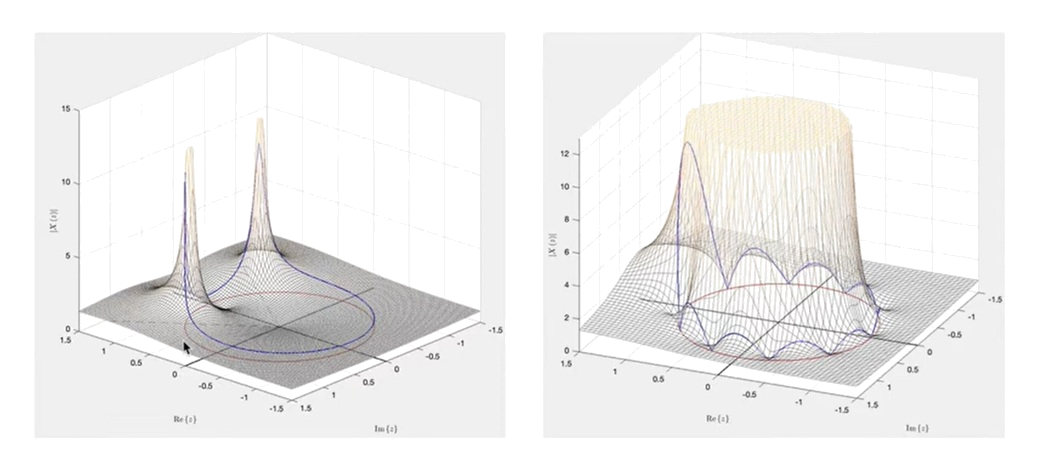
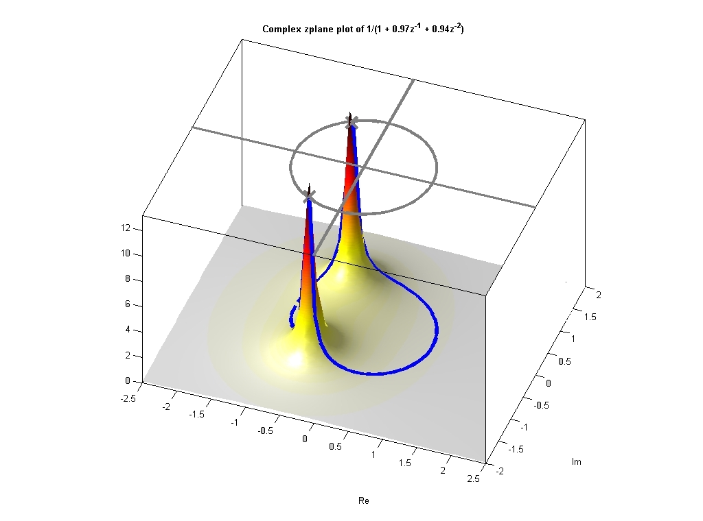
The function is a surface rather than just a curve or a graph of a single dimensional variable
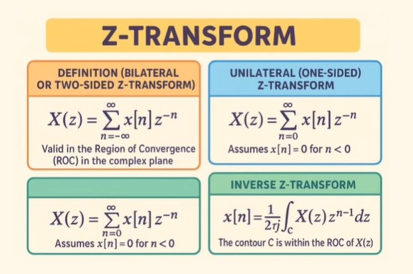
Bilateral Z-transform Pair
Although Z transforms are rarely solved in practice using integration, we will provide the bilateral Z transform pair here for purposes of discussion and derivation. These define the forward and inverse Z transformations. Notice the similarities between the forward and inverse transforms. This will give rise to many of the same symmetries found in Fourier analysis.
Z Transform
\(X(z)=\sum_{n=-\infty}^\infty x\lbrack n\rbrack z^{-n}\)
Inverse Z Transform
\(x\lbrack n\rbrack=\frac1{2\pi j}\oint_rX(z)z^{n-1}\mathrm dz\)
unilateral Z-transform
\(X(z)=\sum_{n=0}^\infty x\lbrack n\rbrack z^{-n}\)
which is useful for solving the difference equations with nonzero initial conditions. This is similar to the unilateral Laplace Transform in continuous time.
\(Z\{x\lbrack k\rbrack\}=X(z)=\sum_{k=0}^\infty x\lbrack k\rbrack z^{-k}\)
[Ex] \(x\lbrack k\rbrack=1,\;for\;k=0,1,2,\cdots\)
\(Z\{x\lbrack k\rbrack\}=\sum_{k=0}^\infty x\lbrack k\rbrack z^{-k}=1+z^{-1}+z^{-2}+\cdots+{\left.z^{-n}\right|}_{n\rightarrow\infty}\)
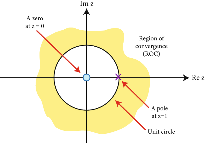
\(=\frac1{1-z^{-1}}=\frac z{z-1},\;\left|z\right|>1\)
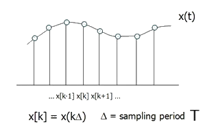
Sampling data
\(x_s(t)=\sum_{k=0}^\infty x(t)\delta(t-kT)\)
\(\sum_{k=-\infty}^\infty\delta(t-kT)=\sum_{k=-\infty}^\infty c_ke^{jk\omega_0T}\)
\(X_s(s)=\mathcal F\{\sum_{k=0}^\infty x(t)\delta(t-kT)\}\)
\(=\sum_{k=0}^\infty x(kT)\mathcal F\{\delta(t-kT)\}\)
\(=\sum_{k=0}^\infty x(kT)e^{-skT}\)
The Laplace Transform
\(X(s)\triangleq{\mathcal L}_s\{x\}\triangleq\int_0^\infty x(t)e^{-st}\operatorname dt\)
\(X(j\omega)=\int_0^\infty x(t)e^{-j\omega t}dt\)
Relation to the Z-Transform
\(X_d(z)\triangleq\sum_{n=0}^\infty x_d(nT)z^{-n}\)
If we define \(z=e^{sT}\)
\(X_d(e^{sT})\triangleq\sum_{n=0}^\infty x_d(nT)e^{-snT}\)
As the sampling interval \(T\) goes to zero,
\(\lim_{T\rightarrow0}X_d(e^{sT})T=\lim_{T\rightarrow0}\sum_{n=0}^\infty x_d(t_n)e^{-st_n}T\)
\(=\int_0^\infty{x_d(t)e^{-st}}\operatorname dt\triangleq X(s)\)
where \(t_n=nT\) and \(\triangle t\triangleq t_{n+1}-t_n=T\)
The Z-Transform (times the sampling interval \(T\)) of a discrete time signal \(x_d(nT)\) approaches, as \(T\rightarrow0\), the Laplace Transform of the the underly-ing continuous-time signal \(x_d(t)\)
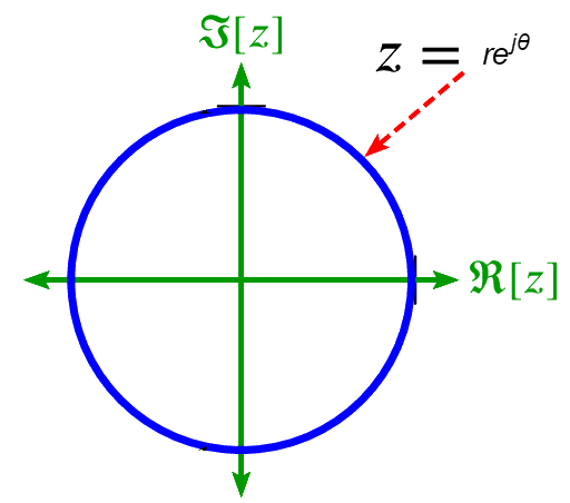
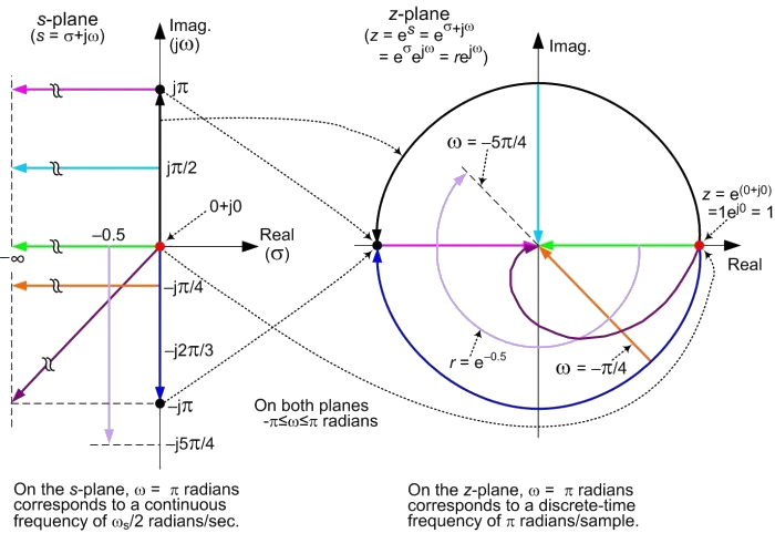
Note that the \(z\) plane and \(s\) plane are related by
\[z=e^{sT}\]
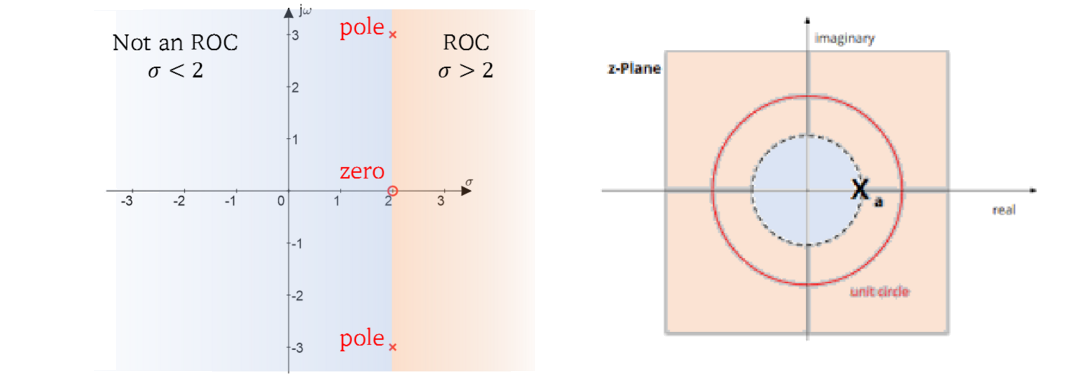
In particular, the discrete-time frequency axis \(\omega_d\in(-\frac{\pi}T,\frac{\pi}T)\) and continuous-time frequency axis \(\omega_a\in(-\infty,\infty)\) are related by
\[e^{j\omega_dT}=e^{j\omega_aT}\]
Laplace Transform
\(x_s(t)\rightarrow X_s(s)=\sum_{k=0}^\infty x\lbrack k\rbrack{(e^{-sT})}^k\)
\(\sum_{k=0}^\infty x(t)\delta(t-kT)\)
Z-Transform
\(x\lbrack k\rbrack\rightarrow X(z)=\sum_{k=0}^\infty x\lbrack k\rbrack z^{-k}\)
\(X_s(s)={\left.X(z)\right|}_{z=e^{sT}}\)
Z-Transform for discrete signals
(1) The Unit Impulse Signal (Delta function)
\(x\lbrack k\rbrack=\delta\lbrack k\rbrack=\left\{\begin{array}{l}1,\;k=0\\0,\;k\neq0\end{array}\right.\)
\(X(z)=\mathcal Z\{x\lbrack k\rbrack\}=\sum_{k=0}^\infty x\lbrack k\rbrack z^{-k}=z^{-0}=1\)
(2) The Exponential Signal
\(x\lbrack k\rbrack=a^k,\;a>0\)
\(X(z)=\sum_{k=0}^\infty x\lbrack k\rbrack z^{-k}=\sum_{k=0}^\infty a^kz^{-k}\)
\(=\sum_{k=0}^\infty{(\frac za)}^{-k}=\frac1{1-{(\frac za)}^{-1}},\;\vert(\frac za)\vert>1\)
\(=\frac{\frac za}{\frac za-1}=\frac z{z-a},\;\vert z\vert>a\)
(3) The Unit Step Signal
\(s\lbrack k\rbrack=1,\;k=0,1,2,\cdots\)
\(X(z)=\frac z{z-1},\;\vert z\vert>1\)
(4) The Natural Exponential Signal
\(x\lbrack k\rbrack=e^{\alpha k}={(e^\alpha)}^k,\;\alpha\in R\)
\(X(z)=\frac z{z-e^\alpha},\;\vert z\vert>e^\alpha\)
(5) The Complex Exponential Signal
\(x\lbrack k\rbrack=e^{j\beta k},\;\beta\in R\)
\(X(z)=\frac z{z-e^{j\beta}},\;\vert z\vert>\vert e^{j\beta}\vert=1\)
(6) The Trigonometric Signal
\(\mathcal Z\{e^{j\beta k}\}=\mathcal Z\{\cos\beta k\}+j\mathcal Z\{\sin\beta k\}\)
\(X(z)=\frac z{z-e^{j\beta}}=\frac z{(z-\cos\beta)-j\sin\beta}\)
\(=\frac{z\lbrack(z-\cos\beta)+j\sin\beta\rbrack}{{(z-\cos\beta)}^2+\sin^2\beta}\)
\(=\frac{z(z-\cos\beta)+jz\sin\beta}{z^2-2\cos\beta z+1}\)
\(\therefore\mathcal Z\{\cos\beta k\}=\frac{z(z-\cos\beta)}{z^2-2\cos\beta z+1}\)
\(\mathcal Z\{\sin\beta k\}=\frac{z\sin\beta}{z^2-2\cos\beta z+1}\)
(7) The Unit Ramp Sequence
\(r\lbrack k\rbrack=k\)
\(R(z)=\sum_{k=0}^\infty kz^{-k}=z^{-1}+2z^{-2}+3z^{-3}+\cdots\)
\(zR(z)=1+2z^{-1}+3z^{-2}+4z^{-3}+\cdots\)
\(zR(z)-R(z)=1+z^{-1}+z^{-2}+z^{-3}+\cdots=\frac1{1-z^{-1}}=\frac z{z-1},\;\vert z\vert>1\)
\(R(z)=\frac z{{(z-1)}^2},\;\vert z\vert>1\)
Z-Transform Properties
(1) Linearity
\(\mathcal Z\{ax\lbrack k\rbrack+by\lbrack k\rbrack\}=a\mathcal Z\{x\lbrack k\rbrack\}+b\mathcal Z\{y\lbrack k\rbrack\}\)
(2) Time Shifting
m-delayed signal \(x\lbrack k-m\rbrack,\;m>0\)
\(\mathcal Z\{x\lbrack k-m\rbrack\}=\sum_{k=0}^\infty x\lbrack k-m\rbrack z^{-k}\)
\(let\;p=k-m\)
\(=\sum_{p=-m}^\infty x\lbrack p\rbrack z^{-(p+m)}=\sum_{p=0}^\infty x\lbrack p\rbrack z^{-(p+m)}=z^{-m}\sum_{p=0}^\infty x\lbrack p\rbrack z^{-p}\)
\(\mathcal Z\{x\lbrack k-m\rbrack\}=z^{-m}X(z)\)
m-advanced signal \(x\lbrack k+m\rbrack,\;m>0\)
\(\mathcal Z\{x\lbrack k+m\rbrack\}=z^mX(z)-z^m\underbrace{\sum_{p=0}^{m-1}x\lbrack p\rbrack z^{-p}}_{x\lbrack0\rbrack,x\lbrack1\rbrack,\cdots,x\lbrack m-1\rbrack,\;initial\;values}\)
\(\mathcal Z\{x\lbrack k+m\rbrack\}=\sum_{k=0}^\infty x\lbrack k+m\rbrack z^{-k}\)
\(q=k+m,\;k=q-m,\;q:m\rightarrow\infty\)
\(\mathcal Z\{x\lbrack k+m\rbrack\}=\sum_{q=m}^\infty x\lbrack q\rbrack z^{-q+m}\)
\(=z^m\sum_{q=m}^\infty x\lbrack q\rbrack z^{-q}\)
\(={z^m(}\sum_{q=0}^\infty x\lbrack q\rbrack z^{-q}-\sum_{q=0}^{m-1}x\lbrack q\rbrack z^{-q})\)
\(=z^m\sum_{q=0}^\infty x\lbrack q\rbrack z^{-q}-\sum_{q=0}^{m-1}x\lbrack q\rbrack z^{m-q}\)
\(=z^mX(z)-(x\lbrack0\rbrack z^m+x\lbrack1\rbrack z^{m-1}+\cdots+x\lbrack m-1\rbrack z)\)
Time Shifting Property of Z-Transform
Statement – The time shifting property of Z-transform states that if the sequence \(\mathrm{\mathit{x\left ( n \right )}}$ is shifted by n0 in time domain, then it results in the multiplication by \(\mathrm{\mathit{z^{-n_{\mathrm{0}}}}}\) in the z-domain. Therefore, if
\(\mathrm{\mathit{x\left ( n \right )\overset{ZT}{\leftrightarrow}X\left ( z \right );\: \: \mathrm{ROC}\mathrm{\, =\, }\mathit{R} }}\)
With zero initial conditions.
Then, according to the time shifting property,
\(\mathrm{\mathit{x\left ( n-n_{\mathrm{0}} \right )\overset{ZT}{\leftrightarrow}z^{-n_{\mathrm{0}}}\, X\left ( z \right )}}\)
With ROC = R, except for the possible addition and deletion of ? = 0 or ? = ∞
Proof
From the definition of the Z-transform, we have,
\(\mathrm{\mathit{Z\left [ x\left ( n \right ) \right ]\mathrm{\, =\, }X\left ( z \right )\mathrm{\, =\, }\sum_{n\mathrm{\, =\, }-\infty }^{\infty }x\left ( n \right )z^{-n}}}\)
\(\mathrm{\mathit{\therefore Z\left [ x\left ( n-n_{\mathrm{0}} \right ) \right ]\mathrm{\, =\, }\sum_{n\mathrm{\, =\, }-\infty }^{\infty }x\left ( n-n_{\mathrm{0}} \right )z^{-n}}}\)
Substituting \(\mathrm{\mathit{\left ( n-n_{\mathrm{0}}\right )=m }}\) in the above summation, then we have,
\(\mathrm{\mathit{Z\left [ x\left ( n-n_{\mathrm{0}} \right ) \right ]\mathrm{\, =\, }\sum_{m\mathrm{\, =\, }-\infty }^{\infty }x\left ( m \right )z^{-\left ( m\mathrm{\, +\, }n_{\mathrm{0}} \right )}}}\)
\(\mathrm{\mathit{\Rightarrow Z\left [ x\left ( n-n_{\mathrm{0}} \right ) \right ]\mathrm{\, =\, }z^{-n_{\mathrm{0}}}\sum_{m\mathrm{\, =\, }-\infty }^{\infty }x\left ( m \right )z^{-m}\mathrm{\, =\, }z^{-n_{\mathrm{0}}}X\left ( z \right ) }}\)
\(\mathrm{\mathit{\therefore Z\left [ x\left ( n-n_{\mathrm{0}} \right ) \right ]\mathrm{\, =\, }z^{-n_{\mathrm{0}}}X\left ( z \right )}}\)
Also, it can be represented as,
\(\mathrm{\mathit{x\left ( n-n_{\mathrm{0}} \right )\overset{ZT}{\leftrightarrow}z^{-n_{\mathrm{0}}}X\left ( z \right )}}\)
Similarly, if signal is advanced in time, then according to the time shifting property, we get,
\(\mathrm{\mathit{x\left ( n\mathrm{\, +\, }n_{\mathrm{0}} \right )\overset{ZT}{\leftrightarrow}z^{n_{\mathrm{0}}}X\left ( z \right )}}\)
Also, if the initial conditions are not neglected, then
-
The time shift property for time delay is,
\(\mathrm{\mathit{Z\left [ x\left ( n-n_{\mathrm{0}} \right ) \right ]\mathrm{\, =\, }z^{-n_{\mathrm{0}}}X\left ( z \right )\mathrm{\, +\, }z^{-n_{\mathrm{0}}}\sum_{p\mathrm{\, =\, }\mathrm{1}}^{n_{\mathrm{0}}}x\left ( -p \right )z^{p}}}\)
-
The time shifting property for time advance is,
\(\mathrm{\mathit{Z\left [ x\left ( n\mathrm{\, +\, }n_{\mathrm{0}} \right ) \right ]\mathrm{\, =\, }z^{n_{\mathrm{0}}}X\left ( z \right )-z^{n_{\mathrm{0}}}\sum_{p\mathrm{\, =\, }\mathrm{0}}^{n_{\mathrm{0}}-\mathrm{1}}x\left ( p \right )z^{-p}}}\)
(3) Premultiplying \(a^{-k}\)
\(\mathcal Z\{a^{-k}x\lbrack k\rbrack\}=\sum_{k=0}^\infty a^{-k}x\lbrack k\rbrack z^{-k}\)
\(=\sum_{k=0}^\infty x\lbrack k\rbrack{(az)}^{-k}\)
\(=X(az)\)
[Ex] \(\mathcal Z\{b^k\cos\beta k\}=\mathcal Z\{{(\frac1b)}^{-k}\cos\beta k\}\)
\(={\left.\frac{z^2-z\cos\beta}{z^2-2z\cos\beta+1}\right|}_{z\rightarrow\frac zb}\)
\(=\frac{{(\frac zb)}^2-(\frac zb)\cos\beta}{{(\frac zb)}^2-2(\frac zb)\cos\beta+1}\)
\(=\frac{z^2-zb\cos\beta}{z^2-2zb\cos\beta+b^2}\)
\(\mathcal Z\{\cos\beta k\}=\frac{z^2-z\cos\beta}{z^2-2z\cos\beta+1}\)
\(=\frac{z(z-\cos\beta)}{{(z-\cos\beta)}^2+\sin^2\beta}\)
\(\mathcal Z\{\sin\beta k\}=\frac{z\sin\beta}{{(z-\cos\beta)}^2+\sin^2\beta}\)
\(\mathcal Z\{b^k\sin\beta k\}=\frac{(\frac zb)\sin\beta}{{(\frac zb)}^2-2(\frac zb)\cos\beta+1}=\frac{zb\sin\beta}{z^2-2zb\cos\beta+b^2}\)
(4) Premultiplying \(k^n\)
\(X(z)=\sum_{k=0}^\infty x\lbrack k\rbrack z^{-k}\)
\(\frac d{dz}X(z)=-\sum_{k=0}^\infty kx\lbrack k\rbrack z^{-(k+1)}\)
\(=-\frac1z\sum_{k=0}^\infty kx\lbrack k\rbrack z^{-k}\)
\(=-\frac1z\mathcal Z\{kx\lbrack k\rbrack\}\)
\(\therefore\mathcal Z\{kx\lbrack k\rbrack\}=-z\frac d{dz}X(z)\)
\(\mathcal Z\{k^2x\lbrack k\rbrack\}=\mathcal Z\{k(kx\lbrack k\rbrack)\}\)
\(=-z\frac d{dz}(-z\frac d{dz}X(z))\)
\(={(-z\frac d{dz})}^2X(z)\)
\(\Rightarrow\mathcal Z\{k^nx\lbrack k\rbrack\}{(-z\frac d{dz})}^nX(z)\)
(5) Initial Value Theorem
\(X(z)=\sum_{k=0}^\infty x\lbrack k\rbrack z^{-k}\)
\(=x\lbrack0\rbrack+x\lbrack1\rbrack z^{-1}+x\lbrack2\rbrack z^{-2}+\cdots\)
\(X(\infty)=x\lbrack0\rbrack,\;x\lbrack0\rbrack={\left.X(z)\right|}_{z\rightarrow\infty}\)
(6) Final Value Theorem
\(X(z)\;poles\;located\;within\;the\;unit\;circle\)
\(\int_{-\infty}^\infty f(t)e^{-st}\operatorname dt\;includes\;imaginary\;axis\)
\(\sum_{k=0}^\infty x\lbrack k\rbrack z^{-k}\;includes\;unit\;circle\)
\(\mathcal Z\{x\lbrack k+1\rbrack-x\lbrack k\rbrack\}\)
\(=\sum_{k=0,\;N\rightarrow\infty}^Nx\lbrack k+1\rbrack z^{-k}-\sum_{k=0,\;N\rightarrow\infty}^Nx\lbrack k\rbrack z^{-k}\)
\(=zX(z)-x\lbrack0\rbrack z-X(z)\)
\(if\;z\rightarrow1,\;then\)
\(\sum_{k=0,\;N\rightarrow\infty}^Nx\lbrack k+1\rbrack z^{-k}-\sum_{k=0,\;N\rightarrow\infty}^Nx\lbrack k\rbrack z^{-k}=zX(z)-X(z)-x\lbrack0\rbrack\)
\(\therefore x\lbrack N+1\rbrack-\cancel{x\lbrack0\rbrack}={\left.zX(z)-X(z)-\cancel{x\lbrack0\rbrack}\right|}_{z\rightarrow1,\;N\rightarrow\infty}\)
\(\Rightarrow x\lbrack N+1\rbrack={\left.(z-1)X(z)\right|}_{z\rightarrow1,\;N\rightarrow\infty}\)
\(\Rightarrow x\lbrack\infty\rbrack={\left.(z-1)X(z)\right|}_{z\rightarrow1}\)
\(\therefore x\lbrack\infty\rbrack=\lim_{z\rightarrow1}(z-1)X(z)\)
(7) Convolution
\(h\lbrack k\rbrack\ast u\lbrack k\rbrack=\sum_{m=0}^\infty h\lbrack k-m\rbrack u\lbrack m\rbrack\)
\(=\sum_{m=0}^kh\lbrack k-m\rbrack u\lbrack m\rbrack\)
\(\mathcal Z\{h\lbrack k\rbrack\ast u\lbrack k\rbrack\}=\sum_{k=0}^\infty\sum_{m=0}^\infty h\lbrack k-m\rbrack u\lbrack m\rbrack z^{-k}\)
\(=\sum_{m=0}^\infty(\sum_{k=0}^\infty h\lbrack k-m\rbrack z^{-(k-m)})u\lbrack m\rbrack z^{-m}\)
\(=\sum_{m=0}^\infty H(z)u\lbrack m\rbrack z^{-m}\)
\(=H(z)U(z)\)
[Ex] \(X(z)=\frac z{z-0.9}\)
\(X_1(z)=\frac1{z-0.9}=z^{-1}X(z)\)
\(x\lbrack k\rbrack=0.9^k\)
\(x_1\lbrack k\rbrack=0.9^{k-1}\;(k\geq1)\)
\(\frac z{z-0.9}=\frac1{1-(0.9z^{-1})}\)
\(\frac1{1-r}=1+r+r^2+r^3+\dots\)
\(\frac z{z-0.9}=\underbrace1_{\delta\lbrack k\rbrack}+(0.9z^{-1})+{(0.9)}^2z^{-2}+{(0.9)}^3z^{-3}+\dots\)
\(x\lbrack0\rbrack=1,\;x\lbrack1\rbrack=0.9,\;x\lbrack2\rbrack={0.9}^2\)
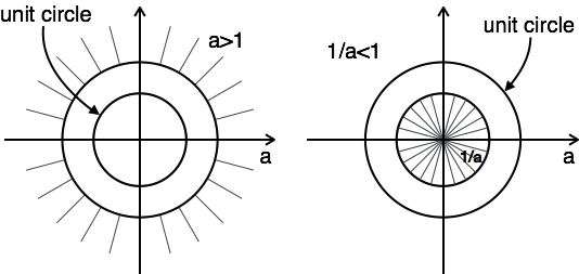
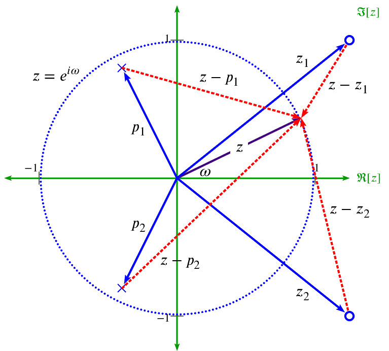
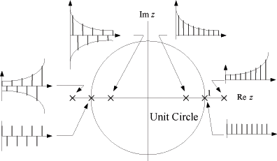
The frequency response of a filter is determined by the interaction of a unit vector rotating around the unit circle with the poles and zeros of the filter.
The unit vector at rotation ω=0 corresponds to DC (0Hz).
The unit vector at rotation ω=π (180°) corresponds to Fs/2 or the Nyquist frequency.
When the tip of the unit vector gets close to a zero, the filter magnitude response is pushed downwards because zero is a root of the numerator polynomial. When the tip of the unit vector gets close to a pole, the filter magnitude response is pushed upwards because a pole is a root of the denominator polynomial.
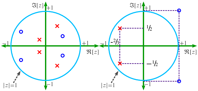
Pole-zero locations are important for:
Wavelets
Symlets
B-splineis
Nyquist frequency
The Nyquist frequency (also called the folding frequency), named after Harry Nyquist, is a characteristic of a sampler. It converts a continuous function or signal into a discrete sequence, it is the frequency you need to sample an analog signal at in order to reconstruct it adequately. The Nyquist frequency is defined as 2*(freq. of original signal).
Usually in practical cases, 5 to 10 times frequency of original signal is selected.
| Property | Signal | Z-Transform | Region of Convergence |
|---|---|---|---|
| Linearity | \(\alpha x_{1}(n)+\beta x_{2}(n)\) | \(\alpha X_{1}(z)+\beta X_{2}(z)\) | At least \(\mathrm{ROC}_{1} \cap \mathrm{ROC}_{2}\) |
| Time shifing | \(x(n-k)\) | \(z^{-k}X(z)\) | \(\mathrm{ROC}\) |
| Time scaling | \(x(n/k)\) | \(X(z^k)\) | \(\mathrm{ROC}^{1/k}\) |
| Z-domain scaling | \(a^{n}x(n)\) | \(X(z/a)\) | \(|a| \: \mathrm{ROC}\) |
| Conjugation | \(\overline{x(n)}\) | \(\overline{X}(\overline{z})\) | \(\mathrm{ROC}\) |
| Convolution | \(x_{1}(n) * x_{2}(n)\) | \(X_{1}(z) X_{2}(z)\) | At least \(\mathrm{ROC}_{1} \cap \mathrm{ROC}_{2}\) |
| Differentiation in z-Domain | \([n x[n]]\) | \(-\frac{d}{d z} X(z)\) | \(\mathrm{ROC}\) = all \(\mathbb{R}\) |
| Parseval's Theorem | \(\sum_{n=-\infty}^{\infty} x[n] \mathrm{x}*[n]\) | \(\int_{-\pi}^{\pi} F(z) \mathbf{F} *(z) d z\) | \(\mathrm{ROC}\) |
| Signal, x[n] | Z-transform, X(z) | Region of Convergence (ROC) |
|---|---|---|
| \(\delta[n]\) | \(1\) | all \(z\) |
| \(\delta[n-m]\) | \(z^{-m}\) | all \(z \neq 0\) |
| \(u[n]\) | \(\Large \frac{1}{1-z^{-1}}\) | \(\lvert z \rvert > 1\) |
| \(a^{n}u[n]\) | \(\Large \frac{1}{1-az^{-1}}\) | \(\lvert z \rvert > \lvert a \rvert\) |
| \(na^{n}u[n]\) | \(\Large \frac{az^{-1}}{(1-az^{-1})^2}\) | \(\lvert z \rvert > \lvert a \rvert\) |
| \(-a^{n} u[-n-1]\) | \(\Large \frac{1}{1-az^{-1}}\) | \(\lvert z \rvert < \lvert a \rvert\) |
| \(-na^{n} u[-n-1]\) | \(\Large \frac{az^{-1}}{(1-az^{-1})^2}\) | \(\lvert z \rvert < \lvert a \rvert\) |
| \(\cos (\omega_0 n) u[n]\) | \(\Large \frac{1 - z^{-1} cos(\omega_0)}{1-2z^{-1}cos (\omega_0) + z^{-2}}\) | \(\lvert z \rvert > 1\) |
| \(\sin (\omega_0 n)u[n]\) | \(\Large \frac{z^{-1} sin(\omega_0)}{1-2z^{-1}cos(\omega_0) + z^{-2}}\) | \(\lvert z \rvert > 1\) |
| \(a^{n}\cos (\omega_0 n) u[n]\) | \(\Large \frac{1 - az^{-1} cos(\omega_0)}{1-2az^{-1}cos (\omega_0) + a^{2}z^{-2}}\) | \(\lvert z \rvert > \lvert a \rvert \) |
| \(a^{n}\sin (\omega_0 n)u[n]\) | \(\Large \frac{az^{-1} sin(\omega_0)}{1-2az^{-1}cos(\omega_0) + a^{2}z^{-2}}\) | \(\lvert z \rvert > \lvert a \rvert \) |