


Mathematics Yoshio Sep 8th, 2024 at 8:00 PM 8 0
微積分 Calculus
CalculusGreek Alphabet

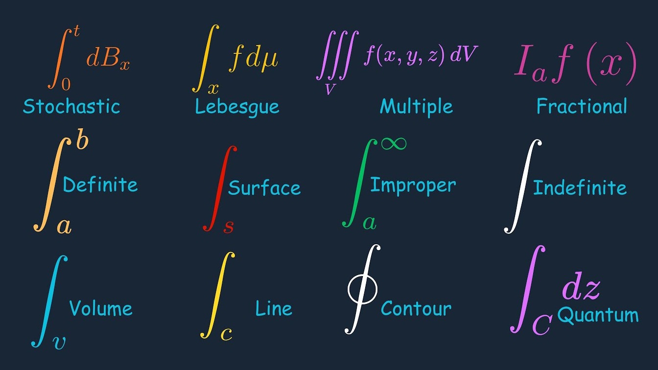
Every type of Integral
Every type of Derivative
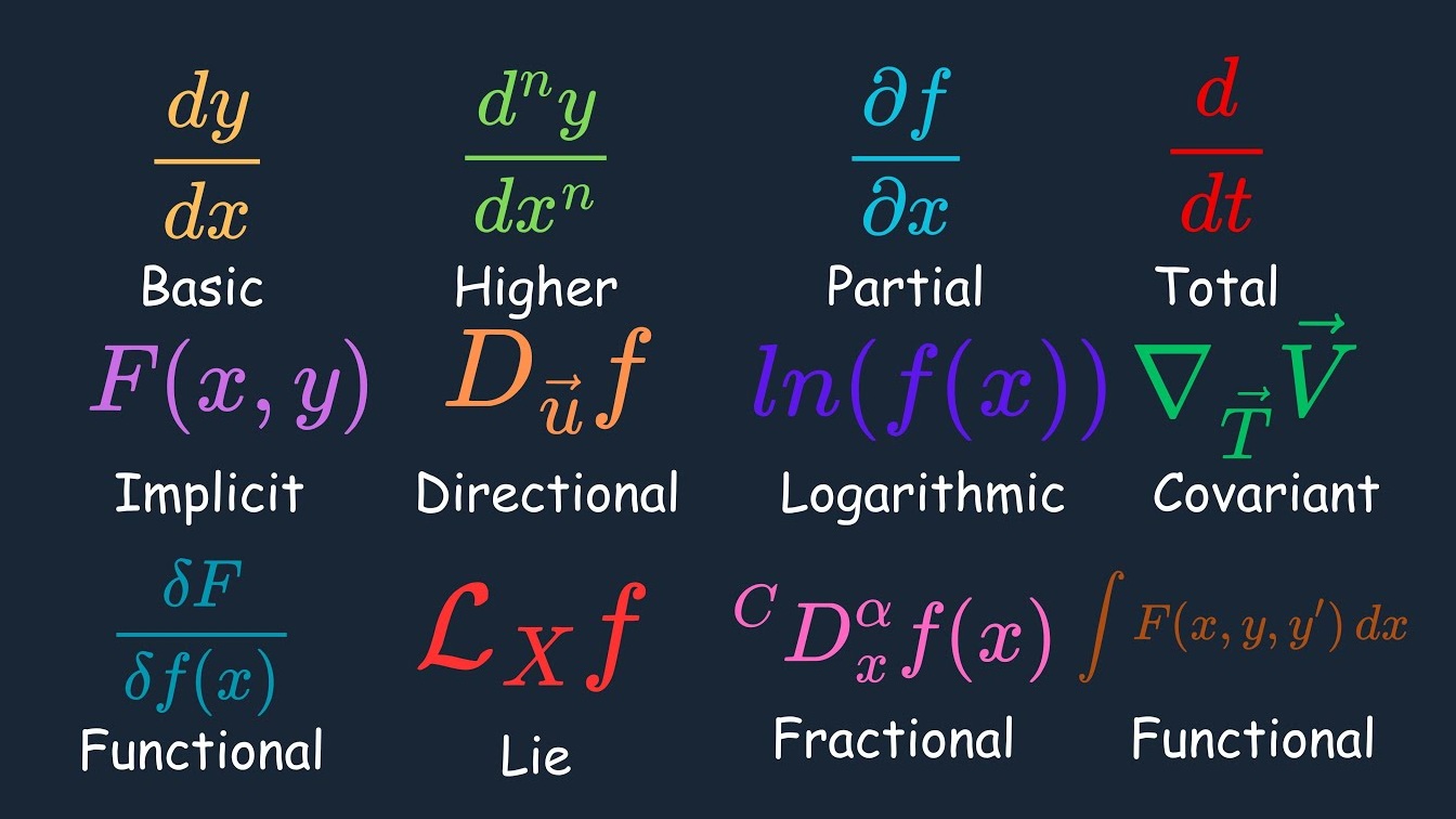
quantum derivative
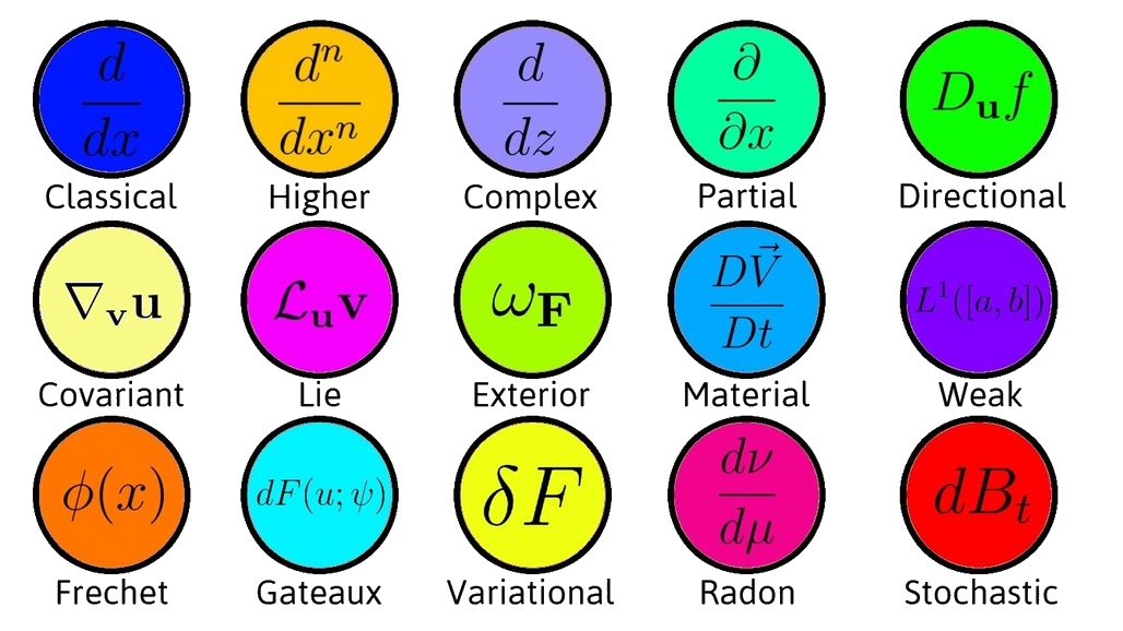
Directional derivative
\(\mathcal R^n\rightarrow\mathcal R\;in\;the\;direction\;of\;\overset\rightharpoonup v\;is\)
\[D_\overset\rightharpoonup vf=\lim_{h\rightarrow0}\frac{f(\overset\rightharpoonup x+h\overset\rightharpoonup v)-f(\overset\rightharpoonup x)}h\]

Fundamental Theorem of Calculus
Integration
\(g(t)=\int_a^tf(\tau)\operatorname d\tau,\;(a\leq t\leq b)\)
\(\dot g(t)=f(t)\)


\(\dot g(t)=\lim_{\triangle t\rightarrow0}\frac{g(t+\triangle t)-g(t)}{\triangle t}\)
\(=\lim_{\triangle t\rightarrow0}\frac{f(t)\triangle t}{\triangle t}=f(t)\)
Antiderivative
\(\int_a^bf(\tau)\operatorname d\tau=h(b)-h(a)\)
\(h(t)=\int_\alpha^tf(\tau)\operatorname d\tau\)
\(\dot h(t)=f(t)\)
\(h(b)-h(a)=\int_\alpha^bf(\tau)\operatorname d\tau-\int_\alpha^af(\tau)\operatorname d\tau=\int_a^bf(\tau)\operatorname d\tau\)
Ex
\(g(t)=\int_a^tf(\tau,t)\operatorname d\tau\)
\(\dot g(t)=f(t,t)+\int_a^t\frac\partial{\partial t}\int f(\tau,t)\operatorname d\tau\)
\(f(\tau,t)=t^2+2\tau t\)
\(g(t)=\int_{-3}^t(t^2+2\tau t)\operatorname d\tau\)
\(g(t)=\left.(t^2\tau+t\tau^2)\right|_{-3}^t\)
\(=2t^3+3t^2-9t\)
\(\dot g(t)=6t^2+6t-9\)
(a) \(f(t,t)=t^2+2t^2=3t^2\)
\(\frac\partial{\partial t}f(\tau,t)=2t+2\tau\)
(b) \(\int_{-3}^t\frac\partial{\partial t}f(\tau,t)\operatorname d\tau=\int_{-3}^t(2t+2\tau)\operatorname d\tau\)
\(=\left.(2t\tau+\tau^2)\right|_{-3}^t=2t^2+t^2+6t-9\)
(a)+(b) \(\dot g(t)=6t^2+6t-9\)
Derivatives Functions Rules
The Sum and Difference Rules
\( \frac d{dx}\left[f\left(x\right)+g\left(x\right)\right]=\frac d{dx}f\left(x\right)+\frac d{dx}g\left(x\right)\)
\( \frac d{dx}\left[f\left(x\right)-g\left(x\right)\right]=\frac d{dx}f\left(x\right)-\frac d{dx}g\left(x\right)\)
\(h\left(x\right)=f\left(x\right)+g\left(x\right)\)
\(\frac d{dx}h\left(x\right)\)
\(=\lim\limits_{\triangle x\rightarrow\infty}\frac{h\left(x+\triangle x\right)-h\left(x\right)}{\triangle x}\)
\(=\lim\limits_{\triangle x\rightarrow\infty}\frac{\left[f\left(x+\triangle x\right)+g\left(x+\triangle x\right)\right]-\left[f\left(x\right)+g\left(x\right)\right]}{\triangle x}\)
\(=\lim\limits_{\triangle x\rightarrow\infty}\frac{\left[f\left(x+\triangle x\right)-f\left(x\right)\right]+\left[g\left(x+\triangle x\right)-g\left(x\right)\right]}{\triangle x}\)
\(=\lim\limits_{\triangle x\rightarrow\infty}\frac{f\left(x+\triangle x\right)-f\left(x\right)}{\triangle x}+\lim\limits_{\triangle x\rightarrow\infty}\frac{g\left(x+\triangle x\right)-g\left(x\right)}{\triangle x}\)
\(=\frac d{dx}f\left(x\right)+\frac d{dx}g\left(x\right)\)
The Product Rule
\(\frac d{dx}\left[f\left(x\right)\cdot g\left(x\right)\right]=g\left(x\right)\cdot\frac d{dx}f\left(x\right)+f\left(x\right)\cdot\frac d{dx}g\left(x\right)\)
The Quotient Rule
\(D{\textstyle\left({\displaystyle\textstyle\frac fg}\right)}=\frac{g\cdot D\left(f\right)-f\cdot D\left(g\right)}{g^2}\)
\(D{\textstyle\left({\displaystyle\textstyle\frac fg}\right)}\)
\(=D\left(f\cdot g^{-1}\right)\)
\(=f\cdot D\left(g^{-1}\right)+D\left(f\right)\cdot g^{-1}\)
\(=-f\cdot g^{-2}\cdot D\left(g\right)+D\left(f\right)\cdot g^{-1}\)
\(=-f\cdot g^{-2}\cdot D\left(g\right)+D\left(f\right)\cdot g\cdot g^{-2}\)
\(=\frac{g\cdot D\left(f\right)-f\cdot D\left(g\right)}{g^2} \)
The Chain Rule
\[\frac{dy}{dx}=\frac{dy}{du}{}\frac{du}{dx}\]
Suppose that we have two functions \(f(x)\) and \(g(x)\) and they are both differentiable.
If we define \(F(x) = (f∘g)(x)\) then the derivative of \(F(x)\) is,
\[F^{\prime}{(x)}=f^{\prime}{({g{(x)}})}{}g^{\prime}{(x)}\]
If we have \(y = f(u)\) and \(u = g(x)\) then the derivative of \(y\) is,
\[\frac{dy}{dx}=\frac{dy}{du}{}\frac{du}{dx}\]
Partial Integration
\(\frac d{dx}\lbrack f(x)\cdot g(x)\rbrack\;=\;g(x)\cdot\frac d{dx}f(x)+f(x)\cdot\frac d{dx}g(x)\)
\(\int\left\{\frac d{dx}\lbrack f(x)\cdot g(x)\rbrack\right\}\;dx\)
\(=\int\lbrack g(x)\cdot\frac d{dx}f(x)+f(x)\cdot\frac d{dx}g(x)\rbrack\;dx\)
\(=\int\lbrack g(x)\cdot\frac d{dx}f(x)\rbrack dx+\int\lbrack f(x)\cdot\frac d{dx}g(x)\rbrack dx\)
\(f(x)\cdot g(x)=\int\lbrack g(x)dx\rbrack\frac d{dx}f(x)+\int\lbrack f(x)dx\rbrack\frac d{dx}g(x)\)
\(f\cdot g\;=\;\int g\cdot\operatorname df+\int f\cdot\operatorname dg\)
\(\int f\cdot\operatorname dg\;=f\cdot g-\;\int g\cdot\operatorname df\)
\(\int u\operatorname dv=uv-\int v\operatorname du\)
Tabular Integration
Repeated integration by parts, also called the DI method of Hindu method
Considering a second derivative of \(v\) in the integral on the LHS of the formula for partial integration suggests a repeated application to the integral on the RHS:

Extending this concept of repeated partial integration to derivatives of degree \(n\) leads to

| Step | Procedure |
|---|---|
| Step 1 | In the product comprising the function \(f\), identify the polynomial and denote it \(F(x)\). Denote the other function in the product by \(G(x)\). |
| Step 2 | Create a table of \(F(x)\) and \(G(x)\), and successively differentiate F(x) until you reach \(0\). Successively integrate \(G(x)\) the same amount of times. |
| Step 3 | Negate every second entry under \(F(x)\). |
| Step 4 | Construct the integral by taking the product of \(F(x)\) and the first integral of \(G(x)\), then add the product of \(F′(x)\) times the second integral of \(G(x)\), then add the product of \(F′′(x)\) times the third integral of \(G(x)\), etc… |
LIATE rule
Whichever function comes first in the following list should be \(u\):
| Abbreviation | FunctionType | Examples |
|---|---|---|
| L | Logatithmic functions | \(\ln(x),\;\log_2(x),\;etc\) |
| I | Inverse trigonometric functions | \(\tan^{-1}(x),\;\sin^{-1}(x),\;etc\) |
| A | Algebraic functions | \(x,\;3x^3,\;5x^{21},\;etc\) |
| T | Trigonometric functions | \(\cos(x),\;\tan(x),\;sech(x),\;etc\) |
| E | Exponential functions | \(e^x,\;7^x,\;etc\) |
L'Hôpital's rule
If \(\lim_{x \rightarrow a}f(x) = 0\) and \(\lim_{x \rightarrow a}g(x) = 0\)
or \(\lim_{x\rightarrow a}\vert f(x)\vert=\infty\) and \(\lim_{x\rightarrow a}\vert g(x)\vert=\infty\)
\(\lim_{x \rightarrow a}\frac{f(x)}{g(x)} = \lim_{x \rightarrow a}\frac{f'(x)}{g'(x)}\)
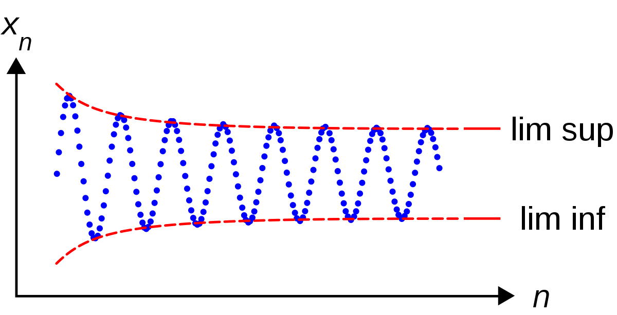
In calculus, the infimum and supremum are mathematical concepts that generalize the minimum and maximum of finite sets. They are used in real analysis, including the definition of the Riemann integral and the construction of real numbers.
Definition: The infimum (inf) of a set is the greatest lower bound of the set, while the supremum (sup) is the least upper bound.
Notation: The infimum of a set is denoted as inf A and the supremum is denoted as sup A.
Existence: The infimum or supremum of a set only exists if it is a finite real number. If a set is not bounded from above, then sup A = ∞. If a set is not bounded from below, then inf A = -∞.
Uniqueness: If the infimum or supremum of a set exists, it is unique.
Partial Integration Applications
Antiderivatives
Polynomials and trigonometric functions
Exponentials and trigonometric functions
Gamma function identity
Green's first identity
https://en.wikipedia.org/wiki/Integration_by_parts
Integration by parts can be extended to functions of several variables by applying a version of the fundamental theorem of calculus to an appropriate product rule. There are several such pairings possible in multivariate calculus, involving a scalar-valued function u and vector-valued function (vector field) V.