


Mathematics Yoshio Sep 8th, 2023 at 8:00 PM 8 0
電路學
Electrical Circuits
An electric circuit is an interconnection of electrical elements.
The law of conservation of charge states that charge can neither be created nor destroyed, only transferred. Thus, the algebraic sum of the electric charges in a system does not change.
A direct current (dc) flows only in one direction and can be constant or time varying.
An alternating current (ac) is a current that changes direction with respect to time.
[Ex] the output of a rectifier (dc) such as i(t) = ∣5 sin(377t)∣ amps or a sinusoidal current (ac) such as i(t) = 160 sin(377t) amps.
Voltage (Potential difference)
The voltage \(v_{ab}\) between two points \(a\) and \(b\) in an electric circuit is the energy (or work) needed to move a unit charge from \(b\) to \(a\); mathematically,
\(v_{ab}\triangleq\frac{dw}{dq}\)
where \(w\) is energy in joules (J) and \(q\) is charge in coulombs (C).
1 volt = 1 joule/coulomb = 1 newton-meter/coulomb
Power and Energy
Power is the time rate of expending or absorbing energy, measured in watts (W).
\(p\triangleq\frac{dw}{dt}\)
\(p=\frac{dw}{dt}=\frac{dw}{dq}\frac{dq}{dt}=vi\)
The power \(p\) is a time-varying quantity and is called the instantaneous power.
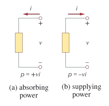
passive sign convension

Passive device
Active device
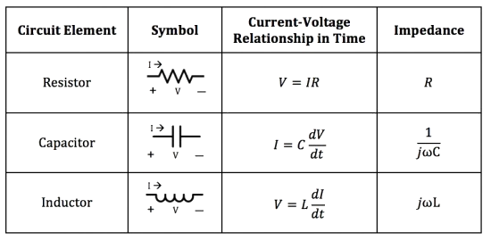
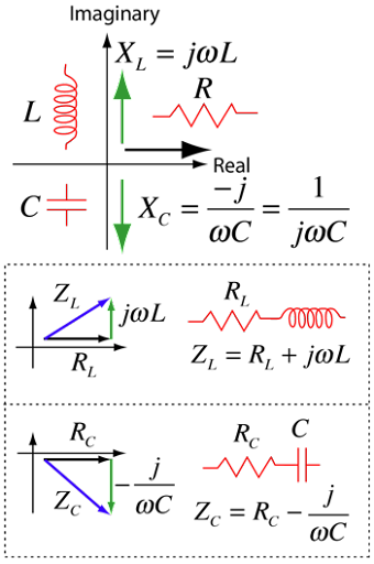
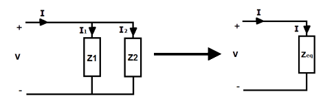
Impedance 阻抗
The real part of impedance is resistance(電阻), while the imaginary part is reactance(電抗). Ideal inductors and capacitors have a purely imaginary reactive impedance:
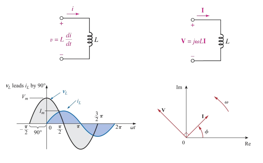
電感 Inductance
The impedance of inductors increases as frequency increases,
\(Z_L={\mathrm{jω}L}\)
The inductance of an electric circuit is one henry when an electric current that is changing at one ampere per second results in an electromotive force of one volt across the inductor:
\[v=L\frac{di}{dt}\]
\[i(t)=\frac1L\int_0^Tv(t)dt+i_0\]
where V(t) is the resulting voltage across the circuit, I(t) is the current through the circuit, and L is the inductance of the circuit.
\(H=\frac{Kg\cdot m^2}{s^2\cdot A^2}=\frac{N\cdot m}{A^2}=\frac{Kg\cdot m^2}{C^2}=\frac J{A^2}=\frac{T\cdot m^2}A=\frac{Wb}A=\frac{V\cdot s}A=\frac{s^2}F=\frac\Omega{Hz}=\Omega\cdot s\)
where: H = henry, kg = kilogram, m = metre, s = second, A = ampere, N = newton, C = coulomb, J = joule, T = tesla, Wb = weber, V = volt, F = farad, Ω = ohm, Hz = hertz
Lenz's law and Faraday's law are both related to the direction of an induced current and the magnitude of the induced electromotive force (EMF). Lenz's law states that the direction of the induced current is always opposite to the change in flux that produced it. Faraday's law states that the magnitude of the induced EMF is directly proportional to the rate of change in the inducing magnetic field.
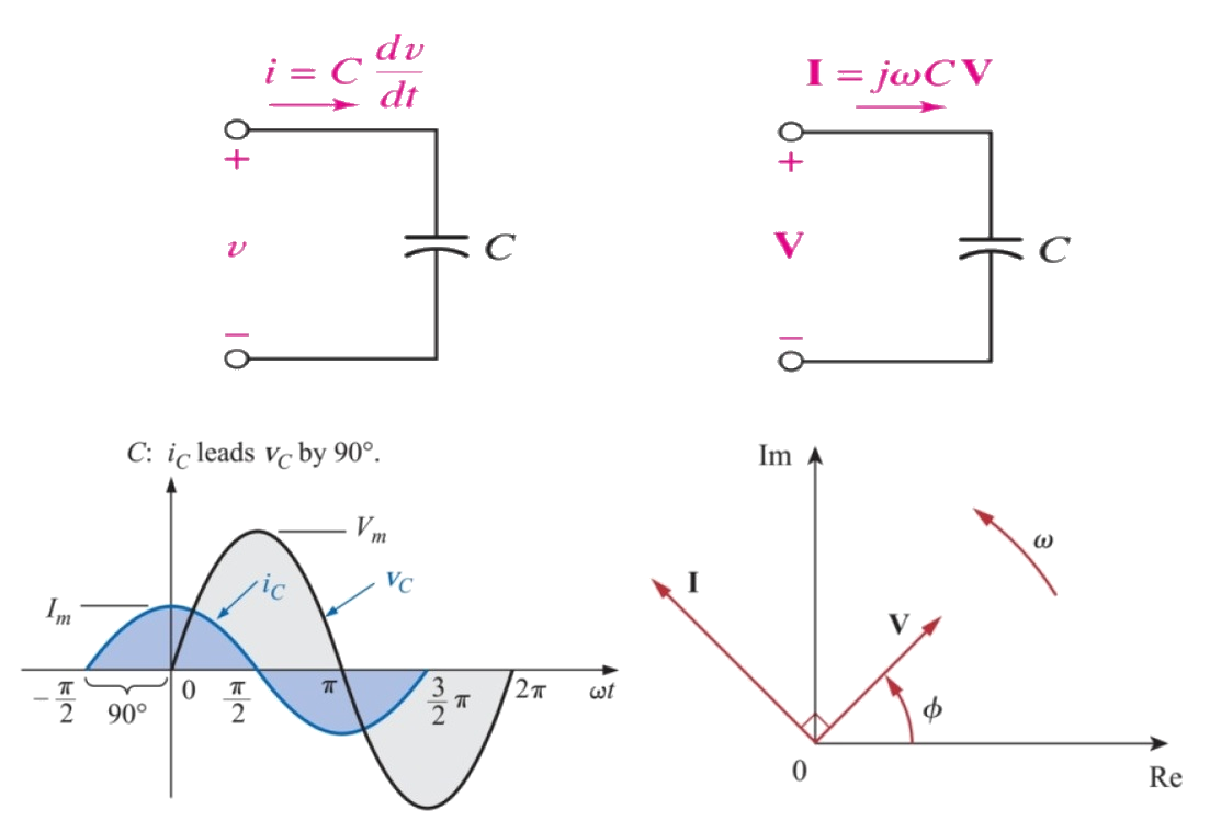
電容 Capacitance
The impedance of capacitors decreases as frequency increases,
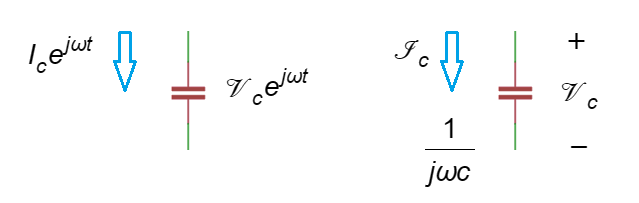
\(Z_C=\frac1{\mathrm{jω}C}\)
The capacitance of a capacitor is one farad when one coulomb of charge changes the potential between the plates by one volt. Equally, one farad can be described as the capacitance which stores a one-coulomb charge across a potential difference of one volt
\[C=\frac QV\]
\[i=C\frac{dv}{dt}\]
\[v(t)=\frac1C\int_0^Ti(t)dt+v_0\]
\(F=\frac{s^4\cdot A^2}{m^2\cdot kg}=\frac{s^4\cdot C^2}{m^2\cdot kg}=\frac CV=\frac{A\cdot s}V=\frac{W\cdot s}{V^2}=\frac J{V^2}=\frac{N\cdot m}{V^2}=\frac{C^2}J=\frac{C^2}{N\cdot m}=\frac s\Omega=\frac1{\Omega\cdot Hz}=\frac S{Hz}=\frac{s^2}H\)
where: F = farad, C = coulomb, V = volt, W = watt, J = joule, N = newton, Ω = ohm, Hz = Hertz, S = siemens, H = henry, A = ampere.
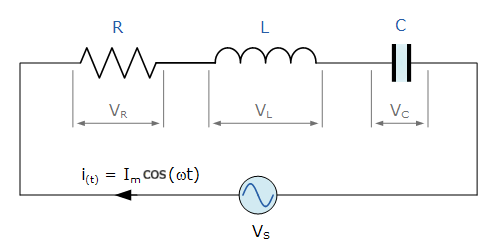
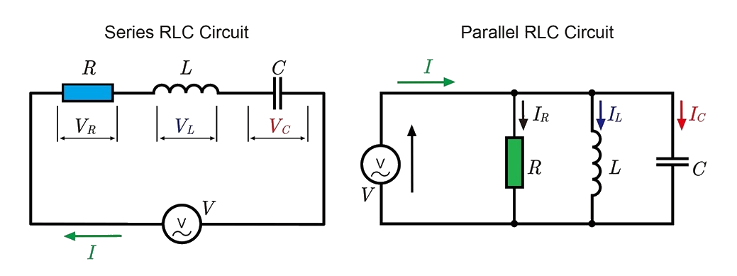
\[V_L(t)=L\frac{\operatorname dI_L}{\operatorname dt}\]
\[I_C(t)=C\frac{\operatorname dV_C}{\operatorname dt}\]
Gauss's Law \(\oint\overset\rightharpoonup E\cdot d\overset\rightharpoonup A=\frac1{\varepsilon_0}Q\)
\(EA=\frac1{\varepsilon_0}Q\)
\(E=\frac Q{\varepsilon_0A}\)
\(+q\;\rightarrow\overset\rightharpoonup{\;F}=q\overset\rightharpoonup E\)
\(w=\overset\rightharpoonup F\cdot\overset\rightharpoonup d=qEd=\triangle PE\;(potential\;energy)\)
\(\frac wq=Ed\equiv V\;(voltage)\)

\(E=-\frac{\partial V}{\partial x}\)
\(V=\frac Q{\varepsilon_0A}d\)
[Ex] \(V=\frac Q{\varepsilon_0A}(d+\triangle d),\;\triangle d\;modulated\;by\;voice\)
\(V=\underbrace{\frac Q{\varepsilon_0A}d}_{V_{dc}}+\underbrace{\lbrack\frac Q{\varepsilon_0A}d\rbrack}_{V_{dc}}(\frac{\triangle d}d)\)
\(V=\underbrace{\frac Q{\varepsilon_0A}d}_{V_{dc}}+\underbrace{v_s(t)}_{V_{ac}}\)
Capacitor
Define \(C\equiv\frac QV\)
\(C=\frac QV=\frac Q{\frac Q{\varepsilon_0A}d}=\varepsilon_0\frac Ad\) geometry
\(d\) is modulated by voice
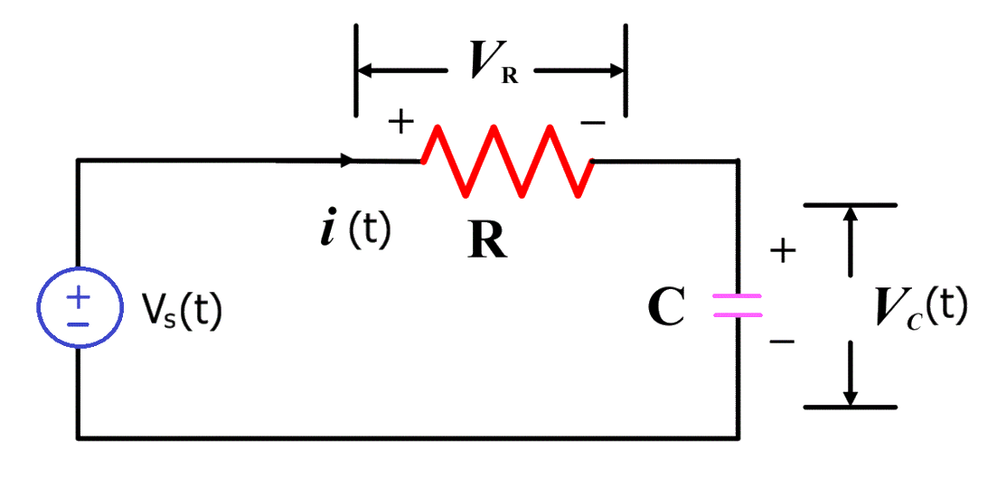
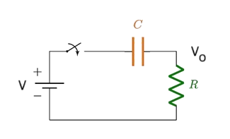
Model the signal source by \(v_s\) in serial with \(R_s\)

\(i=C\frac{dv_o}{dt}\)
\(V_s=RC\frac{dv_o}{dt}+v_o\)

Assume \(v_o=\underbrace{v_{o,t}(t)}_{transient}+\underbrace{v_{o,ss}}_{steady\_state}\)
\(V=RC\frac{dv_{o,t}(t)}{dt}+v_{o,t}(t)+v_{o,ss}\)
\(\left\{\begin{array}{l}RC\frac{dv_{o,t}(t)}{dt}+v_{o,t}(t)=0.\;transient\;solution\;is\;obtained\;by\;removing\;the\;input\;source.\\V=v_{o,ss},\;steady\;state\;solution\;is\;obtained\;by\;\frac d{dt}=0.\;\Rightarrow i_c=0\end{array}\right.\)
\(v_{o,t}(t)=Ae^{st}\;\Rightarrow\;RCsAe^{st}\;+Ae^{st}=0\;\Rightarrow\;(RCs+1)Ae^{st}=0\)
\(\therefore s=-\frac1{RC},\;v_{o,t}(t)=Ae^{-\frac1{RC}t}\)
\(v_o(t)=Ae^{-\frac1{RC}t}+V,\;v_o(0)=0,\;no\;charge\;on\;C\;\Rightarrow A=-V\)
\(v_o(t)=V(1-e^{-\frac1{RC}t})\)
\(\tau\equiv RC\;time\;const\)
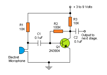
[Ex] \(R=10k\Omega,\;C=1nF\;\Rightarrow\tau=10^4\cdot10^{-9}=10^{-5}\;(s)\)
\(v_o(0)=A+v_o(\infty)\;\Rightarrow A=v_o(0)-v_o(\infty)\)
\(v_o(t)=(v_o(0)-v_o(\infty))e^{-\frac t\tau}+v_o(\infty)\;general\;expression\)
\(\tau=?\;from\;transient\;solution\)
1. remove input source,
\(\tau=C\cdot{\left.(\frac{v_x}{i_x})\right|}_{replace\;C\;by\;v_x}\)
\(v_o(\infty)\Rightarrow let\;C\;''open''\)
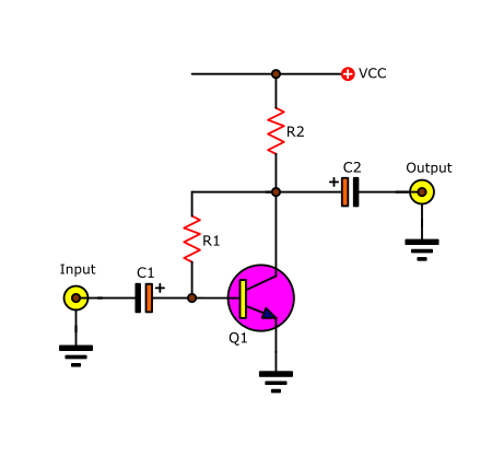
[Ex] \(v_o(t)=(v_o(0)-v_o(\infty))e^{-\frac t\tau}+v_o(\infty)\)
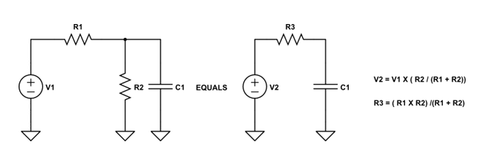
\(let\;C\;''open''\;v_o(\infty)=V\cdot\frac{R_2}{R_1+R_2}\)
\(v_o(0)=0,\;\tau=(R_1\parallel R_2)C\)
\(v_o(t)=V\cdot\frac{R_2}{R_1+R_2}(1-e^{-\frac t{(R_1\parallel R_2)C}})\)
[Ex] \(v_o(t)=(v_o(0)-v_o(\infty))e^{-\frac t\tau}+v_o(\infty)\)
\(let\;C\;''open''\;v_o(\infty)=0\)
\(v_o(0^+)=V,\;\tau=RC\)
\(v_o(t)=Ve^{-\frac t{RC}}\)
Can C block ac signal?

[Ex] \(v_o(t)=(v_o(0)-v_o(\infty))e^{-\frac t\tau}+v_o(\infty)\)
\(let\;C\;''open''\;v_o(\infty)=0\)
\(v_o(0^+)=V\cdot\frac{R_2}{R_1+R_2},\;\tau=(R_1+R_2)C\)
\(v_o(t)=V\cdot\frac{R_2}{R_1+R_2}e^{-\frac t{(R_1+R_2)C}}\)
Inductor
\(V-iR-L\frac{di}{dt}=0\)
\(L\frac{di}{dt}=V-iR\)
\(\frac{di}{dt}=\frac1L(V-iR)\)
\(\frac{di}{dt}=-\frac RL(i-\frac VR)\)
\(at\;t=0,\;i(0)=0,\;\frac{di}{dt}=\frac VL\)
\(at\;t=\infty,\;i(\infty)=\frac VR,\;\frac{di}{dt}=0\)
\(\because\frac{di}{dt}=0=-\frac RL(i-\frac VR),\;i=\frac VR\)
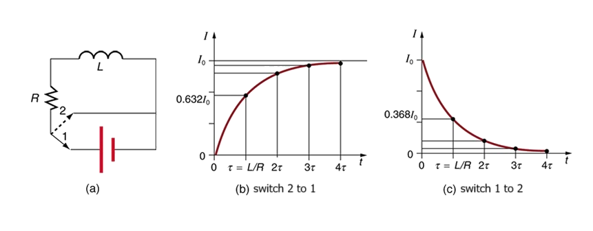
\(i_o(t)=(i_o(0)-i_o(\infty))e^{-\frac t\tau}+i_o(\infty)\;general\;expression\)
\(apply\;\;i(0)=0\;and\;i(\infty)\)
\(i_o(t)=\frac VR(1-e^{-\frac t\tau})\)
\(\tau=\frac LR\)
\(i_o(\infty)\Rightarrow let\;L\;''short''\)
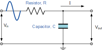
ac voltage charging C
\(v_s(\omega)=V_s\sin\omega t,\;Need\;\tau=RC\;to\;charge\;C\;to\;the\;steady\;state.\)
\(v_o=V_o\sin(\omega t+\theta)\)
\(R=10k\Omega,\;C=1nF,\;\tau=10^{-5}\;sec\)
\(if\;\omega=10^6\pi,\;T=\frac1f=\frac{2\mathrm\pi}\omega=\frac{2\mathrm\pi}{10^6\pi}\Rightarrow\frac T2=10^{-6}\;sec\)


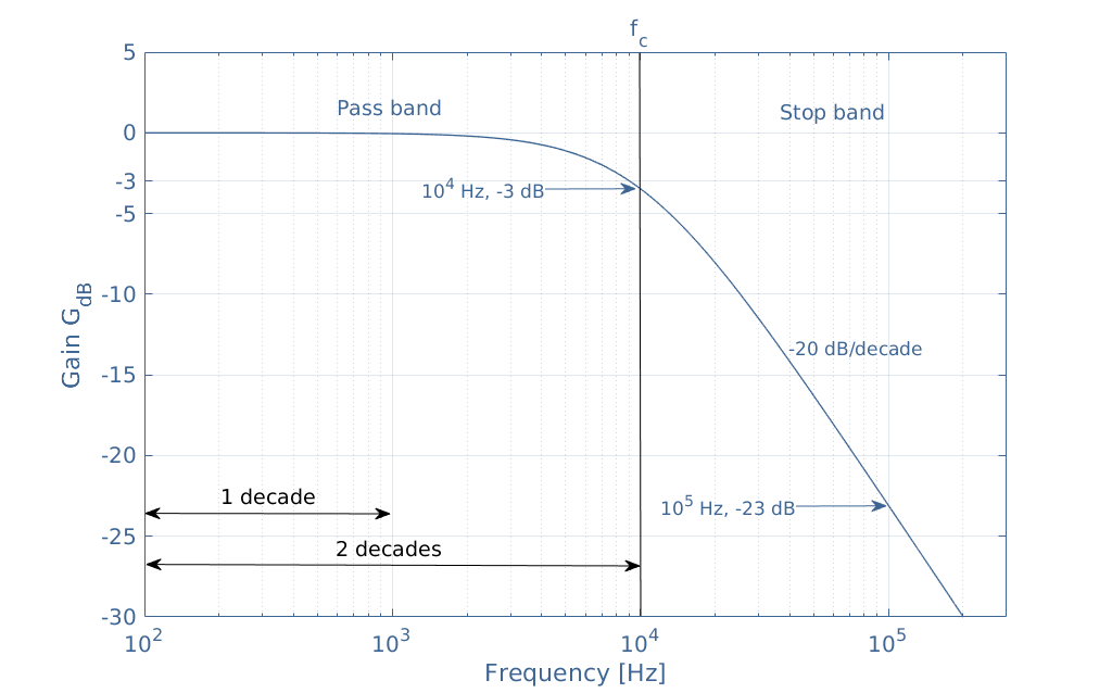
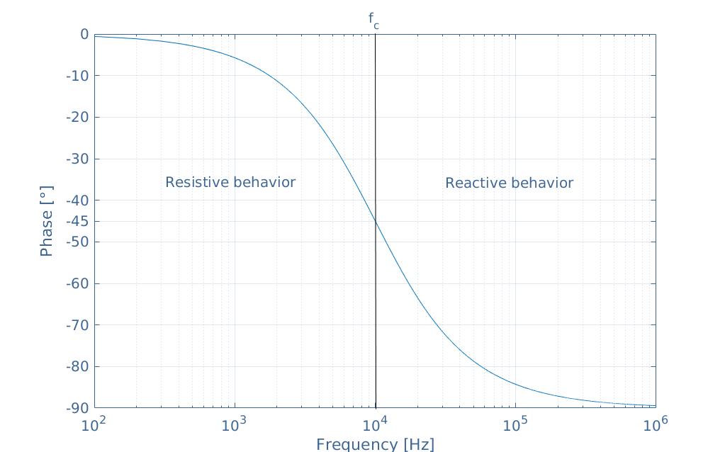
The RC time constant \(\tau=RC\)
Cutoff frequency \(\omega_c=\frac1\tau=2\pi f_c\)
3-dB frequency \(\omega_o\) is also known as the corner frequency, break frequency, or pole frequency

Low pass filter - low frequency C open - high frequency C short.

\(C\equiv\frac QV\Rightarrow i=\frac{dQ}{dt}=c\frac{dv}{dt}\)
\(v=V\sin\omega t\)
\(i=CV\omega\cos\omega t=CV\omega\sin(\omega t+90^\circ)\)
\(R_c=\frac vi=\frac{\cancel V\sin\omega t}{C\cancel V\omega\sin(\omega t+\cancel{90^\circ})}=\frac1{\omega c}\)
\(\frac1{rc}=\omega_o\)
\(v_o=v_s\frac{\frac1{\omega c}}{R+\frac1{\omega c}}\Rightarrow\frac{v_o}{v_s}=\frac1{1+\omega RC}=\frac1{1+{\frac\omega{\omega_o}}}\)
\(R_c\equiv\frac1{\omega c}\rightarrow\infty,\;C:open\;(i_c=0)\)
\(R_c\equiv\frac1{\omega c}\rightarrow0,\;C:short\;(v_c=0)\)

[Ex] voice \(f=20\sim20k,\;\omega=2\pi f=10^2\sim10^5\) allow voice to pass. require \(0.1\omega_o\geq10^5\;\Rightarrow\;\omega_o\geq10^6\)
\(\frac1{RC}\geq10^6\)
\(If\;R=10k,\;\frac1{10^4C}\geq10^6\Rightarrow C\leq\frac1{10^{10}}=0.1nF\)
while filter out high frequency noise
Sample rates were first discussed in the 1940s, as part of the Nyquist-Shannon theorem. This states that any sampling rate must have twice the frequency of the original recording, otherwise the sound is not faithfully reproduced.
The human ear can hear between 20 hertz (20Hz) and 20 kilohertz (20kHz). 44.1kHz is more than twice the top range of human hearing, so will provide a very accurate reproduction according to the theory.
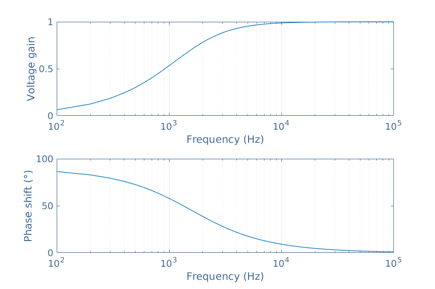
The High Pass Filter Circuit (CR circuit)


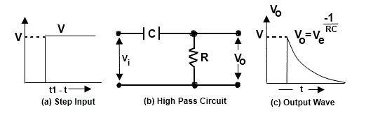
\(v_o=v_s\frac R{\frac1{\omega c}+R}\Rightarrow\frac{v_o}{v_s}=\frac R{\frac1{\omega c}+R}=\frac1{\frac1{\omega RC}+1}=\frac1{1+{\frac{\omega_o}\omega}}\)
\(v_s:\;voice,\;allow\;voice\;to\;pass\), require \(10\omega_o\leq10^2\)
\(\omega_o\leq10\Rightarrow\frac1{RC}\leq10\)
\(10^4C\geq\frac1{10}\Rightarrow C\geq10\mu F\)
C can block DC voltage.
\(\frac1{\omega c}\ll R\;for\;AC\;signal\;\Rightarrow\frac1{\omega c}\ll0.1R\)
\(0.1\omega\geqslant\frac1{RC}\Rightarrow0.1\omega\geqslant\omega_o\)
\(\omega\geqslant10\omega_o\)
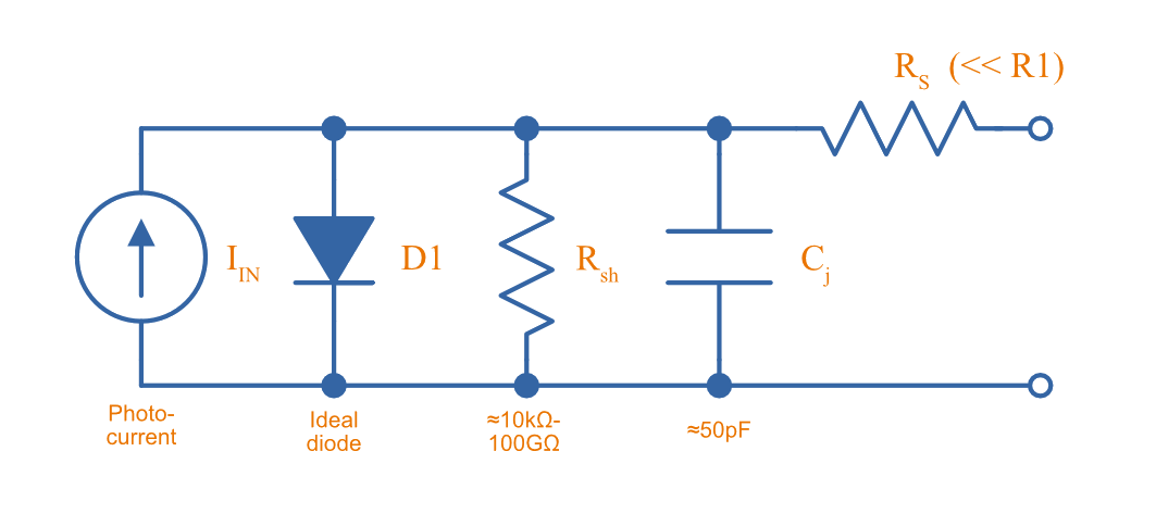
Laser point \(I_L\propto I_{dc}\)
reguire \(\frac1{\omega c}\leq0.1R_L\)
\(60Hz\;ripple\;ac\Rightarrow\frac1{400C}\leq0.1\cdot0.1k\)
\(C\geq\frac14mF\)
C provides a path for noise (AC)

RL filters
\(R\equiv\frac1{\omega C}=\omega L\)

Electrical Impedance
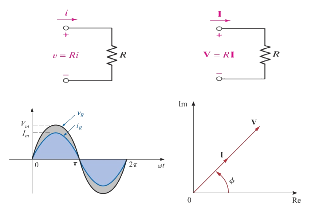
Alternating current, magnitude and phase
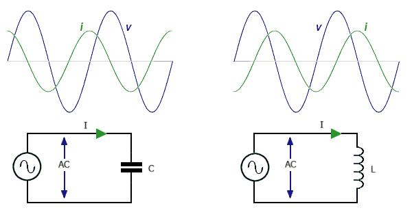
When an alternating current is being used the ratio \(\frac VI\) is not necessarily constant. This is because the voltage and current can peak at different times if the circuit contains components like coils or capacitors.
Impedance Z measures the ratio of the peak voltage to the peak current:
\(Z=\frac{V_{peak}}{I_{peak}}\)
The unit of Z is the ohm (Ω).
Sometimes we break the impedance down into two components. One part has the voltage and current in phase (peaking at the same time), and is the resistance, \(R\). The other part has the current peaking one quarter of a cycle after the voltage, and this is called reactance, \(X\). The impedance is the vector sum of the two:
\(Z=\sqrt{R^2+X^2}\)
The reactance of an inductor is positive \(X_L=\omega L\) and depends on the angular frequency \(\omega=2\pi f\) of the alternating current. The reactance of a capacitor is negative \(X_C=-\frac1{\omega C}\), showing that for a capacitor the current peaks one quarter of a cycle before the voltage.
In more advanced work it is convenient to write the impedance as a complex number with the resistance as the real part and the reactance as the imaginary part \(Z=R+iX\).