In continuous-time Fourier series, periodic signals are represented as sum of complex exponentials. The continuous-time Fourier representation of periodic signal takes a form of infinite series whereas discrete time Fourier representation is of finite series, as a result of this, there is no convergence issue with DTFS.

The Definition of DTFS

The discrete time Fourier series representation is given as
\(x\lbrack n\rbrack=\sum_{n=0}^{N-1}C_ke^{j(\frac{2\pi}N)kn}\)

Where \(C_k\) is Fourier series coeffficient and given as
\(C_k=\frac1N\sum_{n=0}^{N-1}x\lbrack n\rbrack e^{-j(\frac{2\pi}N)kn}\)

Thus \(C_k\) and \(x[n]\) makes discrete time Fourier series coefficient pair
\(x\lbrack n\rbrack\overset{DTFS}\leftrightarrow C_k\)

Features of DTFS

1. Fourier series representation of discrete and periodic signal is also discrete and periodic.
2. \(C_k\) is periodic with \(N\). i.e. \(C_k=C_{k+N}\)
3. Fourier series for discrete time periodic signal is a finite sum defined entirely by the value of signal itset over one period, the series always converges.
4. \(C_k\) repeats every \(2\pi\) interval along \(\Omega\) scale.

Summary Table of DTFS Properties

Discrete Time Fourier Transform

The extension of discrete-time Fourier series for discrete-time aperiodic signals gives discrete-time Fourier transform. The frequency domain description of discrete-time signal is continuous function of \(\Omega\) tha can take any value over continuous interval from \(-\infty\) to \(+\infty\) and it is periodic function of frequency with period \(2\pi\)

The Definition of DTFT

Consider a discrete-time signal \(x[n]\). Its discrete-time Fourier transform (DTFT) is defined as
\({\mathcal F}_{DTFT}\{x(n)\}=X(\Omega)=\sum_{n=-\infty}^\infty x\lbrack n\rbrack e^{-j\Omega n}\)

Where \(\Omega\) is discrete time frequency in "rad/numbers". The transform \(X(\Omega)\) is frequency domain description of \(x[n]\). Thus \(x[n]\) and \(X(\Omega)\) makes Fourier transform pair as
\(\underbrace{x(n)}_{Discrete\;Aperiodic}\xrightarrow{DTFT}\underbrace{X(\Omega)}_{Periodic\;continuous}\)

and the inverse DTFT with maps the frequency domain description \(X(\Omega)\) back into time is given as
\(\mathcal F_{DTFT}^{-1}\{X(\Omega)\}=\frac1{2\pi}\int_{2\pi}X(\Omega)e^{j\Omega n}d\Omega\)

Note some books use different notations \(X(j\omega),\;X(\Omega),\;X(j\Omega),\;X(e^{j\Omega}),\;X(e^{j\omega})\)

Nature of Fourier Spectrum and Periodicity of DTFT

\(X(\Omega)\), the frequency domain representation is continuous function of \(\Omega\) which can take any value over a continuous interval from \(-\infty\) to \(+\infty\), Also, \(X\Omega\) is periodic function of \(\Omega\) with period of \(2\pi\). It follows that

\(X(\Omega)=X(\Omega+2\pi)\)

\(X(\Omega+2\pi)=\sum_{n=-\infty}^\infty x\lbrack n\rbrack e^{-j(\Omega+2\pi)n}=\sum_{n=-\infty}^\infty x\lbrack n\rbrack e^{-j\Omega n}e^{-j2\pi n}\)
\(=\sum_{n=-\infty}^\infty x\lbrack n\rbrack e^{-j\Omega n}=X(\Omega)\)

Distortionless Transmission

In many applications it is required that the output waveform (signal) be a replica of input. Transmission is said to be distortionless if input \(x[n]\) and output \(y[n]\) satisfy the ondition
\[y\lbrack n\rbrack=k\;x\lbrack n-n_0\rbrack\]

where \(k\) is a constant and accounts for scaling in amplitude and \(n_0\) accounts for the delay (in samples) is assumed to be an integer.

Proof of fourier transformation of convolution of two signals

\(\int_{-\infty}^\infty f(t-\tau)g(\tau)\operatorname d\tau\)

\(\int_{-\infty}^\infty\lbrack\underbrace{\int_{-\infty}^\infty f(t-\tau)g(\tau)\operatorname d\tau}_{h(t)}\rbrack e^{-j\omega t}\operatorname dt\)

\(=\int_{-\infty}^\infty\int_{-\infty}^\infty f(t-\tau)g(\tau)e^{-j\omega t}\operatorname d\tau\operatorname dt\)

\(=\int_{-\infty}^\infty g(\tau)\int_{-\infty}^\infty f(t-\tau)e^{-j\omega t}\operatorname dt\operatorname d\tau\)

\(=\int_{-\infty}^\infty g(\tau)\int_{-\infty}^\infty f(s)e^{-j\omega(s+\tau)}\operatorname ds\operatorname d\tau\)

\(=\int_{-\infty}^\infty g(\tau)e^{-j\omega\tau}(\underbrace{\int_{-\infty}^\infty f(s)e^{-j\omega s}\operatorname ds}_{F(\omega)})\operatorname d\tau\)

\(=F(\omega)\underbrace{\int_{-\infty}^\infty g(\tau)e^{-j\omega\tau}\operatorname d\tau}_{G(\omega)}\)

\(=F(\omega)G(\omega)\)

Proof of fourier transformation of multiplication of two signals

\(ℱ\lbrack f(t)g(t)\rbrack=\int_{t=-\infty}^\infty\lbrack f(t)g(t)\rbrack e^{-j\omega t}dt\)

\(\because f(t)=\frac1{2\pi}\int_{\alpha=-\infty}^\infty F(\alpha)e^{j\alpha t}d\alpha\)

\(ℱ\lbrack f(t)g(t)\rbrack=\int_{t=-\infty}^\infty\lbrack\frac1{2\pi}\int_{\alpha=-\infty}^\infty F(\alpha)e^{j\alpha t}d\alpha\rbrack g(t)e^{-j\omega t}dt\)

\(=\frac1{2\pi}\int_{\alpha=-\infty}^\infty F(\alpha)\lbrack\int_{t=-\infty}^\infty g(t)e^{-j(\omega-\alpha)t}dt\rbrack d\alpha\)

\(\because G(\omega)=\int_{t=-\infty}^\infty g(t)e^{-j\omega t}dt\)

and replacing \(\omega\) with \(\omega-\alpha\), we get

\(G(\omega-\alpha)=\int_{t=-\infty}^\infty g(t)e^{-j(\omega-\alpha)t}dt\)

\(ℱ\lbrack f(t)g(t)\rbrack=\frac1{2\pi}\int_{\alpha=-\infty}^\infty F(\alpha)G(\omega-\alpha)d\alpha\)

Finally, we get \(ℱ\lbrack f(t)g(t)\rbrack=\frac1{2\pi}\lbrack F(\omega)\ast G(\omega)\rbrack\)

\(\because x_1(t)\ast x_2(t)=\int_{\tau=-\infty}^\infty x_1(\tau)x_2(t-\tau)d\tau\)

Parseval's theorem

\(E=\int_{-\infty}^\infty f(t)f^\ast(t)\operatorname dt\)

\(=\int_{-\infty}^\infty\left|f(t)\right|^2\operatorname dt\)

\(=\int_{-\infty}^\infty f^2(t)\operatorname dt\)

\(E=\int_{-\infty}^\infty f(t){(\underbrace{\frac1{2\mathrm\pi}\int_{-\infty}^\infty F(\omega)e^{j\omega t}d\omega}_{f(t)})}^\ast dt\)

\(=\int_{-\infty}^\infty f(t)(\frac1{2\mathrm\pi}\int_{-\infty}^\infty F^\ast(\omega)e^{-j\omega t}d\omega)dt\)

\(=\frac1{2\mathrm\pi}\int_{-\infty}^\infty\int_{-\infty}^\infty F^\ast(\omega)f(t)e^{-j\omega t}d\omega dt\)

\(=\frac1{2\mathrm\pi}\int_{-\infty}^\infty F^\ast(\omega)(\int_{-\infty}^\infty f(t)e^{-j\omega t}dt)d\omega\)

\(=\frac1{2\mathrm\pi}\int_{-\infty}^\infty F^\ast(\omega)F(\omega)d\omega\)

\(=\frac1{2\mathrm\pi}\int_{-\infty}^\infty\left|F(\omega)\right|^2d\omega\)

1.The FT of a periodic signal is not one, but (potentially) infinite impulses.

Assume an arbitrary periodic function \(f_T(t)\) with period \(T\) and consider its Fourier series representation in which \(\omega_0=\frac{2\pi}{T}\): \[f_T(t)=\sum_{n=-\infty}^{+\infty}c_n e^{j n \omega_0 t}\] Take the Fourier transform of the sides: \begin{align} \mathcal{F}\{f_T(t)\}=&\mathcal{F}\{\sum_{n=-\infty}^{+\infty}c_n e^{j n \omega_0 t}\}\\ =&c_n\sum_{n=-\infty}^{+\infty}\mathcal{F}\{ e^{j n \omega_0 t}\}\\ =&2\pi c_n\sum_{n=-\infty}^{+\infty}\delta(\omega-n\omega_0) \end{align} This means that the Fourier transform of a periodic signal is an impulse train where the impulse amplitudes are \(2\pi\) times the Fourier coefficients of that signal.

\(\because ℱ^{-1}\{2\mathrm\pi\cdot\delta(\omega-n\omega_0)\}\)

\(=\frac1{2\mathrm\pi}\int_{-\infty}^\infty2\mathrm\pi\cdot\delta(\omega-n\omega_0)e^{j\omega t}dt\)

\(=e^{jn\omega_0t}\)

\(e^{jn\omega_0t}\leftrightarrow2\pi\delta(\omega-n\omega_0)\)

\(\lbrack i\mathit.e\mathit.\mathit,e^{j\omega_0t}\mathit\:x\left(t\right)\overset{FT}{\mathit\leftrightarrow}X\left(\omega\mathit-\omega_0\right)\rbrack\)

\(F\left[1\mathit\:\mathit.e^{jn\omega_0t}\right]\mathit=2\pi\delta\left(\omega\mathit-n\omega_0\right)\)

\[f_T(t)=\sum_{n=-\infty}^{+\infty}c_n e^{j n\omega_0 t}\]

\[F_T(\omega)=2\mathrm\pi\sum_{n=-\infty}^{+\infty}{\mathrm c}_{n}\mathrm\delta(\mathrm\omega-{n\mathrm{ω}}_0)\]

Interpreting the amplitude of signals in fourier transform

Since the sines are orthogonal, the squared magnitude of the coefficients weighting the sines is proportional to the energy of each corresponding sine frequency.

Parseval's theorem

In mathematics, Parseval's theorem usually refers to the result that the Fourier transform is unitary; loosely, that the sum (or integral) of the square of a function is equal to the sum (or integral) of the square of its transform.
In physics, the most general form of this property is more properly called the Plancherel theorem.
In electrical engineering, Parseval's theorem is often written as:

\(\int_{-\infty}^\infty\vert x(t)\vert^2{}\mathrm dt=\frac{\displaystyle1}{\displaystyle2\pi}\int_{-\infty}^\infty\vert X(\omega)\vert^2{}\mathrm d\omega=\int_{-\infty}^\infty\vert X(2\pi f)\vert^2{}\mathrm df\)

The interpretation of this form of the theorem is that the total energy of a signal can be calculated by summing power-per-sample across time or spectral power across frequency.

The magnitude of \(X(ω)\) for a given \(ω\) signifies how much does the signal \(e^{jωt}\) exist in the signal \(x(t)\); indicated as an inner product between \(x(t)\) and \(e^{jωt}\).

For discrete time signals, the theorem becomes:

\(\sum_{n=-\infty}^\infty\vert x\lbrack n\rbrack\vert^2={\frac1{2\pi}}\int_{-\pi}^\pi\vert X_{2\pi}(\phi)\vert^2{\mathrm d}\phi\)

where \(X_{2\pi }\) is the discrete-time Fourier transform (DTFT) of \(x\) and \(\phi\) represents the angular frequency (in radians per sample) of \(x\)

Fourier Transform of Gaussian Signal

For a continuous-time function \(x(t)\), the Fourier transform of \(x(t)\) can be defined as,
\[\mathrm{X(\omega)\:=\:\int_{-\infty }^{\infty} x\left(t\right)\:e^{-j\omega t}\:dt}\]

Gaussian Function The Gaussian function is defined as,
\[\mathrm{g_{a}\left(t\right) \:=\: e^{-at^{2}} ;\:\:for\:all \:t}\]

Therefore, from the definition of Fourier transform, we have,
\[\mathrm X(\mathrm\omega)=\mathcal F(e^{-at^2})=\int_{-\infty}^\infty\mathrm e^{-\mathrm{at}^2}\:\mathrm e^{-\mathrm{jωt}}\:\mathrm{dt}\]

\(\Rightarrow\:\mathrm X\left(\mathrm\omega\right)\:=\:\int_{-\infty}^\infty\:\mathrm e^{-\left(\mathrm{at}^2\:+\:\mathrm{jωt}\right)}\:\mathrm{dt}\)
\(=\int_{-\infty}^\infty\:\mathrm e^{-\left[\mathrm{at}^2\:+\:\mathrm{jωt}+\left(\frac{\mathrm{jω}}{2\sqrt{\mathrm a}}\right)^2\right]}\:\mathrm e^{\left(\frac{\mathrm{jω}}{2\sqrt{\mathrm a}}\right)^2}\mathrm{dt}\)
\(=\mathrm e^{-\left(\frac{\mathrm\omega^2}{4\mathrm a}\right)}\int_{-\infty}^\infty\:\mathrm e^{-\left(\sqrt{\mathrm a}\cdot\mathrm t+\frac{\mathrm{jω}}{2\sqrt{\mathrm a}}\right)^2}\mathrm{dt}\)

Let \(\sqrt{\mathrm a}\cdot\mathrm t+\frac{\mathrm{jω}}{2\sqrt{\mathrm a}}=u\)

Then \(\sqrt{\mathrm a}dt=du\;\Rightarrow\;dt=\frac{du}{\sqrt{\mathrm a}}\)

\(\therefore X(\omega)=\mathrm e^{-\left(\frac{\mathrm\omega^2}{4\mathrm a}\right)}\int_{-\infty}^\infty\:\frac{\mathrm e^{-u^2}}{\sqrt{\mathrm a}}du\)
\(=\frac{\mathrm e^{-\left(\frac{\mathrm\omega^2}{4\mathrm a}\right)}}{\sqrt{\mathrm a}}\int_{-\infty}^\infty\:\mathrm e^{-u^2}du\)

\(\because\int_{-\infty}^\infty\:\mathrm e^{-x^2}dx=\sqrt\pi\)

\(\Rightarrow X(\omega)=\frac{\mathrm e^{-\left(\frac{\mathrm\omega^2}{4\mathrm a}\right)}}{\sqrt{\mathrm a}}\cdot\sqrt\pi=\sqrt{\frac\pi a}\mathrm e^{-\left(\frac{\mathrm\omega^2}{4\mathrm a}\right)}\)

Therefore, the Fourier transform of the Gaussian functions,
\[\mathcal F(e^{-at^2})=\sqrt{\frac\pi a}\mathrm e^{-\left(\frac{\mathrm\omega^2}{4\mathrm a}\right)}\]

\[\mathrm e^{-\mathrm{at}^2}\overset{\mathrm{FT}}\leftrightarrow\sqrt{\frac{\mathrm\pi}{\mathrm a}}\mathrm e^{-\left(\frac{\mathrm\omega^2}{4\mathrm a}\right)}\]

The graphical representation of Gaussian function and its frequency spectrum is,

Fourier Transform of Gaussian Modulated Function

The Gaussian modulated signal is defined as
\(\mathrm x(\mathrm t)=\mathrm e^{-\mathrm{at}^2}{\mathrm{cosω}}_0\mathrm t\)

\(\Rightarrow\mathrm x(\mathrm t)=\mathrm e^{-\mathrm{at}^2}\cdot\frac12(\mathrm e^{{\mathrm{jω}}_0\mathrm t}+\mathrm e^{-{\mathrm{jω}}_0\mathrm t})\)

Therefore the Fourier transform of the Guassian modulated signaled is
\(\mathrm X(\mathrm\omega)=\frac12\mathcal F\{\mathrm e^{-\mathrm{at}^2}\mathrm e^{{\mathrm{jω}}_0\mathrm t}\}+\frac12\mathcal F\{\mathrm e^{-\mathrm{at}^2}\mathrm e^{-{\mathrm{jω}}_0\mathrm t}\}\)

By using frequency shifting property \(\mathrm e^{{\mathrm{jω}}_0\mathrm t}\mathrm x(\mathrm t)\overset{\mathrm{FT}}\leftrightarrow\mathrm X(\mathrm\omega+{\mathrm\omega}_0)\) of Fourier transform, we get
\(\mathcal F\{\mathrm e^{-\mathrm{at}^2}\mathrm e^{{\mathrm{jω}}_0\mathrm t}\}={\left.\mathcal F\{\mathrm e^{-\mathrm{at}^2}\}\right|}_{\mathrm\omega=(\mathrm\omega-{\mathrm\omega}_0)}\)
\(\mathcal F\{\mathrm e^{-\mathrm{at}^2}\mathrm e^{-{\mathrm{jω}}_0\mathrm t}\}={\left.\mathcal F\{\mathrm e^{-\mathrm{at}^2}\}\right|}_{\mathrm\omega=(\mathrm\omega+{\mathrm\omega}_0)}\)

\(\mathcal F\{e^{-at^2}\}=\sqrt{\frac\pi a}\mathrm e^{-\left(\frac{\mathrm\omega^2}{4\mathrm a}\right)}\)

Therefore the Fourier transform of Gaussian modulated function is, \(\mathrm X(\mathrm\omega)=\frac12\{\sqrt{\frac{\mathrm\pi}{\mathrm a}}\mathrm e^{-\left[\frac{\left(\mathrm\omega-{\mathrm\omega}_0\right)^2}{4\mathrm a}\right]}+\sqrt{\frac{\mathrm\pi}{\mathrm a}}\mathrm e^{-\left[\frac{\left(\mathrm\omega+{\mathrm\omega}_0\right)^2}{4\mathrm a}\right]}\}\)

Rectangle Function

\(rect(t)\;=\;\left\{\begin{array}{lc}1&\left|t\right|\leq\frac12\\0&otherwise\end{array}\right.\)

\(\mathrm F(\mathrm\omega)=\int_{-\infty}^\infty\mathrm{rect}(\mathrm t)\mathrm e^{-\mathrm{jωt}}\operatorname d\mathrm t=\int_{-\frac12}^\frac121\cdot\mathrm e^{-\mathrm{jωt}}\operatorname d\mathrm t\)
\(=\left.\frac1{-\mathrm{jω}}\mathrm e^{-\mathrm{jωt}}\right|_{-\frac12}^\frac12\)
\(=\frac1{-\mathrm{jω}}(\mathrm e^{-\mathrm j\frac{\mathrm\omega}2}-\mathrm e^{\mathrm j\frac{\mathrm\omega}2})\)
\(=\frac1{\mathrm\omega/2}\cdot\frac{\mathrm e^{\mathrm j\frac{\mathrm\omega}2}-\mathrm e^{-\mathrm j\frac{\mathrm\omega}2}}{2\mathrm j}\)
\(=\frac{\sin(\mathrm\omega/2)}{(\mathrm\omega/2)}\)

\[\mathrm F(\mathrm\omega)=\mathrm{sinc}(\mathrm\omega/2)\]

The Dirac Delta

\[\delta(t)\Leftrightarrow1\]

DC

\[1\Leftrightarrow2\pi\delta(\omega)\]

Signum (Sign)

\[sgn(t)=u_0(t)-u_0(t-)\Leftrightarrow\frac2{j\omega}\]

The discrete Fourier transform is a transformation that follows from the Fourier transform and is, as its name indicates, adapted for discrete signals.

The Fourier transform

for a function \(f\), its Fourier transform \(\hat f\) is defined by:
\[\hat{f}(\nu) = \int_{-\infty}^{+\infty}f(x)e^{-2i\nu x}\text{d}x\]

Discrete Time Fourier Transform (DTFT)​​

the Fourier transform of a signal is a continuous function of the variable \(\nu\).

1. We sample or discretize the signal to analyze. This means that instead of working on the function that associates the value of the signal with the variable \(x\), we will work on a discrete series of values of the temporal signal. In the case of the DTFT, we sample with a constant step.

2. We window the discretized signal. This means that we keep only a finite number of points of the signal.

3. We sample the Fourier transform of the signal to obtain the discrete Time Fourier Transform.

4. We window the discrete Fourier transform for storage.

A real Gaussian signal. The Fourier transform of a real Gaussian is also a real Gaussian in Frequency.

The signal which will be used as an example

More formally, we have:
\[f(x)=e^{-x^2},\;\widehat{f}(\nu)=\sqrt{\pi}e^{-({πν})^2}\]

Let's first look at the sampling. Mathematically, we can represent the process by the multiplication of the signal \(f\) by a Dirac comb of period \(T\), \(ш_T\). The Dirac comb is defined as follows:

\[ш_T(x) = \sum_{k=-\infty}^{+\infty}\delta(x-kT)\]

With \(δ\) the Dirac distribution. Here is the plot that we can obtain if we represent \(f\) and \(g={ш}_{T}\times f\) together:

The signal and the sampled signal.

The Fourier transform of the new \(g\) function is written,
\[\begin{aligned} \hat{g}(\nu) &= \int_{-\infty}^{+\infty} \sum_{k=-\infty}^{+\infty} \delta(x-kT) f(x) e^{-2i\pi x \nu} \text{d}x \\ &= \sum_{k=-\infty}^{+\infty}\int_{-\infty}^{+\infty}\delta(x-kT) f(x) e^{-2i\pi x \nu}\text{d}x \\ &= \sum_{k=-\infty}^{+\infty}f(kT)e^{-2i\pi kT\nu} \end{aligned}\]

If we put \(f[k]=f(kT)\) the sampled signal \(\nu_{ech} = \frac{1}{T}\) the sampling frequency, we have:

\[\hat{g} = \sum_{k=-\infty}^{+\infty}f[k]e^{-2i\pi k\frac{\nu}{\nu_{\text{ech}}}}\]

If we plot the Fourier transform of the starting signal \(\hat{f}\) and that of the sampled signal \(\hat{g}\), we obtain the following plot:

Fourier transform of the signal and its sampled signal

We can then look at the windowing process. There are several methods that each have their advantages, but we will focus here only on the rectangular window. The principle is simple: we only look at the values of \(f\) for \(x\) between \(-x_0\) and \(+x_0\). This means that we multiply the function \(f\) by a gate function \(Π_{x0}\) which verified,

\[\Pi_{x_0}(x) = \begin{aligned} 1 & \;\text{if}\; x\in[-x_0,x_0] \\ 0 & \;\text{else} \end{aligned} \]

Graphically, here is how we could represent \(h\) and \(f\) together.

Signal sampled and windowed

Concretely, this is equivalent to limiting the sum of the Dirac comb to a finite number of terms. We can then write the Fourier transform of \(h=\Pi_{x_0}\times\Pi ш_T\times f\)

\[\hat{h}(\nu) = \sum_{k=-k_0}^{+k_0}f[k]e^{-2i\pi k\frac{\nu}{\nu_{\text{ech}}}}\]

We can now proceed to the last step: sampling the Fourier transform. Indeed, we can only store a finite number of values on our computer and, as defined, the function \(\hat h\) is continuous. We already know that it is periodic, with period \(ν_{ech}\), so we can store only the values between \(0\) and \(ν_{ech}\). We still have to sample it, and in particular to find the adequate sampling step. It is clear that we want the sampling to be as "fine" as possible, in order not to miss any detail of the Fourier transform! For this we can take inspiration from what happened when we sampled \(f\): its Fourier transform became periodic, with period \(ν_{ech}\). Now the inverse Fourier transform (the operation that allows to recover the signal from its Fourier transform) has similar properties to the Fourier transform. This means that if we sample \(\hat h\) with a sampling step \(v_s\), then its inverse Fourier transform becomes periodic with period \(1/v_s\). This gives a low limit on the values that \(v_s\) can take ! Indeed, if the inverse transform has a period smaller than the width of the window ( \(1/v_s＜2x_0\), then the reconstructed signal taken between \(-x_0\) and \(x_0\) will not correspond to the initial signal \(f\).

So we choose \(v_s=\frac1{2x_0}\) to discretize \(\hat{h}\). We use the same process of multiplication by a Dirac comb to discretize. In this way we obtain the Fourier transform of a new function \(l\):

\[\hat{l}(\nu) = \sum_{n=-\infty}^{+\infty} \delta(\nu-n\nu_s) \sum_{k=-k_0}^{+k_0}f[k]e^{-2i\pi k\frac{n\nu_s}{\nu_{\text{ech}}}}\]

This notation is a bit complicated, and we can be more interested in \(\hat{l}[n]=\hat{l}(n\nu_s)\)

\[\begin{aligned} \hat{l}[n] = \hat{l}(n\nu_s) &=& \sum_{k=-k_0}^{+k_0}f[k]e^{-2i\pi k\frac{n\nu_s}{\nu_{\text{ech}}}}\\ &=& \sum_{k=0}^{N-1}f[k]e^{-2i\pi k\frac{n}{N}} \end{aligned}\]

To get the last line, I re-indexed \(f[k]\) to start at 0, noting \(N\) the number of samples. I then assumed that the window size corresponded to an integer number of samples, i.e. that \(2x_0 = N\times T\), which is rewritten as \(N\times \nu_s = \nu_{ech}\). This expression is the discrete Fourier transform of the signal.

Sampling the Fourier transform of the sampled signal to obtain the discrete Fourier transform

This problem is solved quite simply by windowing the discrete Fourier transform. Since the transform has been periodized by the sampling of the starting signal, it is enough to store one period of the transform to store all the information contained in it. The choice which is generally made is to keep all the points between O and \(ν_{ech}\). This allows to use only positive \(n\), and one can easily reconstruct the plot of the transform if needed by inverting the first and the second half of the computed transform. In practice (for the implementation), the discrete Fourier transform is thus given by :

\[\forall n=0...(N-1),\; \hat{f}[n] = \sum_{k=0}^{N-1}f[k]e^{-2i\pi k\frac{n}{N}}\]

Windowing of the discrete Fourier transform for storage

Calculating the discrete Fourier transform

So we have at our disposal the expression of the discrete Fourier transform of a signal \(f\):

\[\hat{f}[n] = \sum_{k=0}^{N-1}f[k]e^{-2i\pi k\frac{n}{N}}\]

This s the expression of a matrix product which would look like this:
\[\hat{f} = \mathbf{M} \cdot f\]

with
\[\mathbf{M} = \begin{pmatrix} 1 & 1 & 1 & \dots & 1 \\ 1 & e^{-2i\pi 1 \times 1 / N} & e^{-2i\pi 2 \times 1 / N} & \dots & e^{-2i\pi 1\times (N-1)/N} \\ 1 & e^{-2i\pi 1 \times 2 \times 1 / N} & e^{-2i\pi 2 \times 2 / N} & \ddots & \vdots\\ \vdots & \vdots & \ddots & \ddots & e^{e-2i\pi (N-2)\times (N-1) / N}\\ 1 & e^{-2i\pi (N-1) \times 1/N} & \dots & e^{e-2i\pi (N-1) \times (N-2) / N} & e^{-2i\pi (N-1)\times (N-1) / N} \end{pmatrix}\]

Those in the know will notice that this is a Vandermonde matrix on the roots of the unit.

We notice that the sampling of the signal has led to the periodization of its Fourier transform. This leads to an important property in signal processing: the Nyquist-Shanon criterion, and one of its consequences, spectrum aliasing. I let you consult the Wikipedia article about this if you are interested, but you can have a quick idea of what happens if you draw the previous plot with a too large sampling: the bells of the sampled signal transform overlap.

Fourier transform of the signal and its sampled signal, illustrating aliasing

a) Upper-left: A Gaussian function has the same Gaussian shape in both time/space and frequency space
b) Upper-right: sampling Gaussian signal in the time space
c) Lower-left: Gaussian Frequency signal repeated in \(1/T\) as we sample it.
d) Lower-right: Discrete Fourier Transform of Gaussian function

Depiction of a Fourier transform (upper left) and its periodic summation (DTFT) in the lower left corner. The spectral sequences at (c) upper right and (d) lower right are respectively computed from (c) one cycle of the periodic summation of s(t) and (d) one cycle of the periodic summation of the s(nT) sequence. The respective formulas are (c) the Fourier series integral and (d) the DFT summation. Its similarities to the original transform, S(f), and its relative computational ease are often the motivation for computing a DFT sequence.

Fourier Series

Sine-cosine form

\(f(x)=a_0+\sum_{n=1}^\infty a_n\cos(nx)+\sum_{n=1}^\infty b_n\sin(nx)\)

\(\left\{\begin{array}{l}a_0=\frac1{2\pi}\int_{-\pi}^\pi f(x)\operatorname dx\\a_n=\frac1\pi\int_{-\pi}^\pi f(x)\cos(nx)\operatorname dx\\b_n=\frac1\pi\int_{-\pi}^\pi f(x)sin(nx)\operatorname dx\end{array}\right.\)

If \(f(x)\) is a periodic function,
\(f(x)=\sum_{n=0}^\infty\lbrack a_n\cos(\frac{2n\pi}Tx)+b_n\sin(\frac{2n\pi}Tx)\rbrack\)
\(f(x)=a_0+\sum_{n=1}^\infty\lbrack a_n\cos(\frac{2n\pi}Tx)+b_n\sin(\frac{2n\pi}Tx)\rbrack\)

If \(f(x)\)'s period is \(2\pi\)

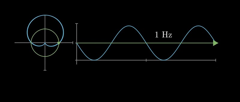
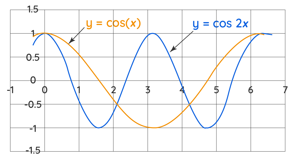
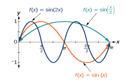
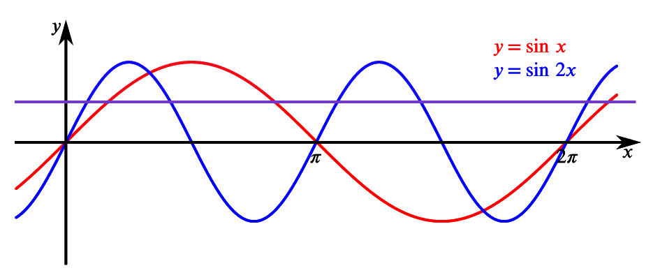
What kind of frequencies should we use?
\(\sin(x),\sin(2x),\sin(\frac x2),\cdots?\;\cos(x),\cos(2x),\cos(\frac x2),\cdots?\) or both?

\(\sin(x),\sin(2x),\sin(nx),\cdots,\;\cos(x),\cos(2x),\cos(nx),\cdots\;\Rightarrow OK\)

\(\sin(\frac x2),\sin(\frac x3),\sin(\frac83x),\cdots,\;\cos(\frac x2),\cos(\frac x3),\cos(\frac83x),\cdots\;\Rightarrow NO\)

\(f(x)=\underbrace{\frac{f(x)+f(-x)}2}_{even}+\underbrace{\frac{f(x)-f(-x)}2}_{odd}\)

\(f(x)=a_0+\sum_{n=1}^\infty a_n\cos(nx)+\sum_{n=1}^\infty b_n\sin(nx),\;N\in\mathcal N,\;a_n,b_n\in\mathcal R\)

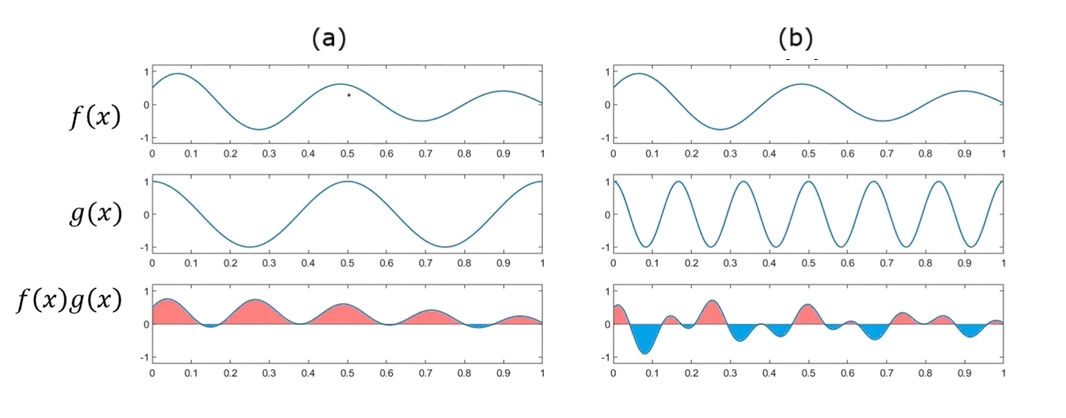
The correlation between two functions can be done by their integral result.

\(\int_a^bf(x)g(x)\operatorname dx,\;\mathcal R\rightarrow\mathcal C\)

How to get \(a_n\) of \(f(x)\)?

[Ex] \(f(x)=a_0+a_1\cos(x)+a_2\cos(2x)+b_1\sin(x)+b_2\sin(2x)\)

\(f(x)=f(x+2\pi)\)

\(\int_{-\pi}^\pi f(x)\operatorname dx=\int_{-\pi}^\pi a_0\operatorname dx=2a_0\pi\;\rightarrow a_0=\frac1{2\pi}\int_{-\pi}^\pi f(x)\operatorname dx\)

\(\int_{-\pi}^\pi f(x)\cos(x)\operatorname dx=a_0\underbrace{\int_{-\pi}^\pi\cos(x)\operatorname dx}_0+a_1\underbrace{\int_{-\pi}^\pi\cos(x)\cos(x)\operatorname dx}_\pi+a_2\underbrace{\int_{-\pi}^\pi\cos(2x)\cos(x)\operatorname dx}_0+b_1\underbrace{\int_{-\pi}^\pi\sin(x)\cos(x)\operatorname dx}_0+b_2\underbrace{\int_{-\pi}^\pi\sin(2x)\cos(x)\operatorname dx}_0\)
\(=a_1\int_{-\pi}^\pi\frac12\lbrack\cos(2x)+1\rbrack\operatorname dx\)
\(\Rightarrow\int_{-\pi}^\pi f(x)\cos(x)\operatorname dx=a_1\pi\;\rightarrow a_1=\frac1\pi\int_{-\pi}^\pi f(x)\cos(x)\operatorname dx\)

\(\Rightarrow a_n=\frac1\pi\int_{-\pi}^\pi f(x)\cos(nx)\operatorname dx,\;n\geq1\)

\(\Rightarrow b_n=\frac1\pi\int_{-\pi}^\pi f(x)\sin(nx)\operatorname dx,\;n\geq1\)

\(f(x)=a_0+\sum_{n=1}^\infty a_n\cos(nx)+\sum_{n=1}^\infty b_n\sin(nx)\)

\(\left\{\begin{array}{l}a_0=\frac1{2\pi}\int_{-\pi}^\pi f(x)\operatorname dx\\a_n=\frac1\pi\int_{-\pi}^\pi f(x)\cos(nx)\operatorname dx\\b_n=\frac1\pi\int_{-\pi}^\pi f(x)sin(nx)\operatorname dx\end{array}\right.\)

\(\left\{\begin{array}{l}a_0=\frac1{2\pi}\int_{-\pi}^\pi f(x)\operatorname dx\\a_n=\frac1\pi\int_{-\pi}^\pi f(x)\cos(nx)\operatorname dx\\b_n=\frac1\pi\int_{-\pi}^\pi f(x)sin(nx)\operatorname dx\end{array}\right.\Rightarrow\left\{\begin{array}{l}\int_{-\pi}^\pi a_0\cos(nx)\operatorname dx=0\\\int_{-\pi}^\pi a_0\sin(nx)\operatorname dx=0\\\int_{-\pi}^\pi\cos(mx)\cos(nx)\operatorname dx\\\int_{-\pi}^\pi\sin(mx)\cos(nx)\operatorname dx\\\int_{-\pi}^\pi\sin(mx)\sin(nx)\operatorname dx\end{array}\right.\)

\(\left.\begin{array}{l}\int_{-\pi}^\pi a_0\cos(nx)\operatorname dx=0\\\int_{-\pi}^\pi a_0\sin(nx)\operatorname dx=0\end{array}\right\}\;\omega=2\pi\)

\(\left.\begin{array}{l}\int_{-\pi}^\pi\cos(mx)\cos(nx)\operatorname dx\\\int_{-\pi}^\pi\sin(mx)\cos(nx)\operatorname dx\\\int_{-\pi}^\pi\sin(mx)\sin(nx)\operatorname dx\end{array}\right\}\left\{\begin{array}{l}m=n\\m\neq n\end{array}\right.\)

\(\int_{-\pi}^\pi\cos(mx)\cos(nx)\operatorname dx=\frac12\int_{-\pi}^\pi\{\cos\lbrack(m+n)x\rbrack+\cos\lbrack(m-n)x\rbrack\}\operatorname dx=\left\{\begin{array}{lc}2\pi&(n=m)=0\\0&n\neq m\\\pi&(n=m)\neq0\end{array}\right.\)

\(\int_{-\pi}^\pi\sin(mx)\cos(nx)\operatorname dx=\frac12\int_{-\pi}^\pi\{\sin\lbrack(m+n)x\rbrack+\sin\lbrack(m-n)x\rbrack\}\operatorname dx=0\)

\(\int_{-\pi}^\pi\sin(mx)\sin(nx)\operatorname dx=-\frac12\int_{-\pi}^\pi\{\cos\lbrack(m+n)x\rbrack-\cos\lbrack(m-n)x\rbrack\}\operatorname dx=\left\{\begin{array}{lc}0&n\neq m\;or\;(n=m)=0\\\pi&(n=m)\neq0\end{array}\right.\)

Apply to any frequency not \(2\pi\)

\(\int_{-L}^L\sin(\frac{n\pi}Lx)\sin(\frac{m\pi}Lx)\operatorname dx=\left\{\begin{array}{ll}0&n\neq m\\0&(n=m)=0\\L&(n=m)\neq0\end{array}\right.\)

\(\int_{-L}^L\cos(\frac{n\pi}Lx)\cos(\frac{m\pi}Lx)\operatorname dx=\left\{\begin{array}{ll}0&n\neq m\\2L&(n=m)=0\\L&(n=m)\neq0\end{array}\right.\)

\(\int_{-L}^L\sin(\frac{n\pi}Lx)\cos(\frac{m\pi}Lx)\operatorname dx=0\)

\(\int_L^L\sin(\frac{n\pi}Lx)\operatorname dx=0\)

\(\int_L^L\cos(\frac{n\pi}Lx)\operatorname dx=0\)

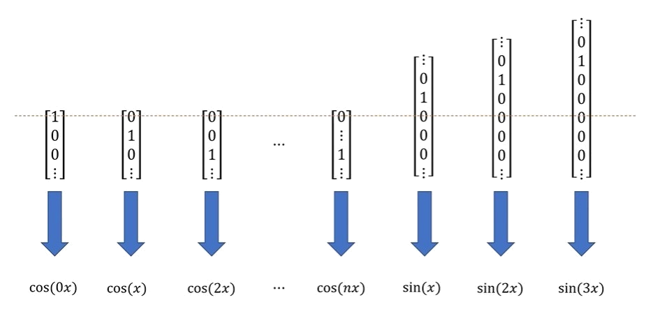
Orthogonal Basis

\(\begin{bmatrix}1\\0\\0\end{bmatrix},\begin{bmatrix}0\\1\\0\end{bmatrix},\begin{bmatrix}0\\0\\1\end{bmatrix}\)

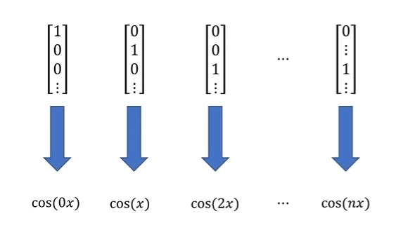
including \(cos(nx)\) and \(sin(nx)\)

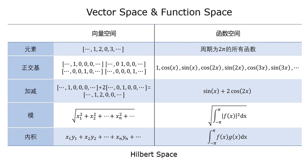
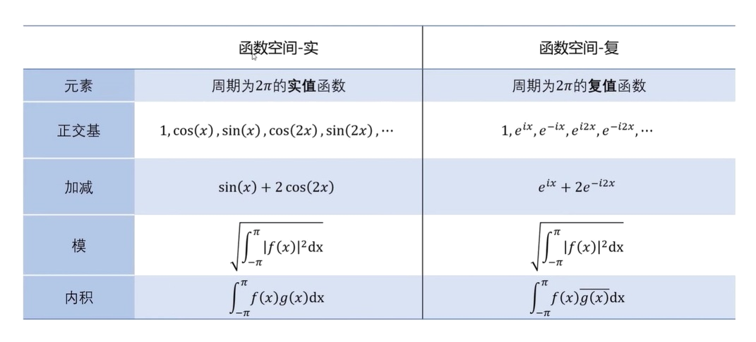
\(\int_{-\pi}^\pi f(x)g(x)\operatorname dx\): inner product of two functions

\(\sqrt{\int_{-\pi}^\pi\left|f(x)\right|^2\operatorname dx}\): norm of a function

Hilbert Space

In mathematics, a Hilbert space is a real or complex inner product space that is also a complete metric space with respect to the metric induced by the inner product. It generalizes the notion of Euclidean space, to infinite dimensions. The inner product, which is the analog of the dot product from vector calculus, allows lengths and angles to be defined. Furthermore, completeness means that there are enough limits in the space to allow the techniques of calculus to be used. A Hilbert space is a special case of a Banach space.

A Hilbert space is a vector space \(H\) with an inner product \(\left\langle f,\;g\right\rangle\) such that the norm defined by
\(|f|=\sqrt{\left\langle f,f\right\rangle}\)

turns \(H\) into a complete metric space.

The overtones of a vibrating string. These are eigenfunctions of an associated Sturm–Liouville problem. The eigenvalues 1, ⁠½, ⅓, ... form the (musical) harmonic series.

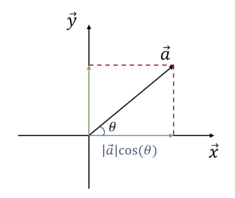
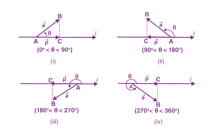
Projection

\(\left\langle\overset\rightharpoonup a,\overset\rightharpoonup x\right\rangle=\left|\overset\rightharpoonup a\right|\left|\overset\rightharpoonup x\right|\cos(\theta)\)

\(Projection\;on\;x-axis:\frac{\left\langle\overset\rightharpoonup a,\overset\rightharpoonup x\right\rangle}{\left|\overset\rightharpoonup x\right|}\)

\(Projection\;on\;y-axis:\frac{\left\langle\overset\rightharpoonup a,\overset\rightharpoonup y\right\rangle}{\left|\overset\rightharpoonup y\right|}\)

Orthogonal basis but not a non-standard basis

\(\cos(x),\;\sin(x),\;\cos(2x),\;\sin(2x),\;\cdots\)

the norm of \(sin(nx)\): \(\sqrt{\int_{-\pi}^\pi\sin^2(nx)\operatorname dx}=\sqrt\pi\)

the norm of \(cos(nx)\): \(\sqrt{\int_{-\pi}^\pi cos^2(nx)\operatorname dx}=\sqrt\pi,\;(n\neq0)\)

the norm of \(1\): \(\sqrt{\int_{-\pi}^\pi1^2\operatorname dx}=\sqrt{2\pi}\)

\(\underbrace{1,\;\cos(x),\;\sin(x),\;\cos(2x),\;\sin(2x),\;\cdots}_{non\;standard\;basis}\;\Rightarrow\underbrace{\frac1{\sqrt{2\pi}},\;\;\frac{\cos(x)}{\sqrt\pi},\;\frac{\sin(x)}{\sqrt\pi},\;\frac{\cos(2x)}{\sqrt\pi},\;\frac{\sin(2x)}{\sqrt\pi},\;\cdots}_{standard\;basis}\)

\(f(x)\) with \(2\pi\) frequency signals projected on \(cos(2x)\) direction

\(\frac{\left\langle f(x),\cos(2x)\right\rangle}{\left|\cos(2x)\right|}=\frac{\int_{-\pi}^\pi f(x)cos(2x)\operatorname dx}{\sqrt{\int_{-\pi}^\pi cos^2(2x)\operatorname dx}}=\frac1{\sqrt\pi}\int_{-\pi}^\pi f(x)cos(2x)\operatorname dx\;\Rightarrow\frac1{\sqrt\pi}\int_{-\pi}^\pi f(x)cos(nx)\operatorname dx\)

\(f(x)\) with \(2\pi\) frequency signals projected on \(cos(2x)\) basis

\(\frac{\left\langle f(x),\cos(2x)\right\rangle}{\left|\cos(2x)\right|^2}=\frac1\pi\int_{-\pi}^\pi f(x)cos(2x)\operatorname dx=a_2\)

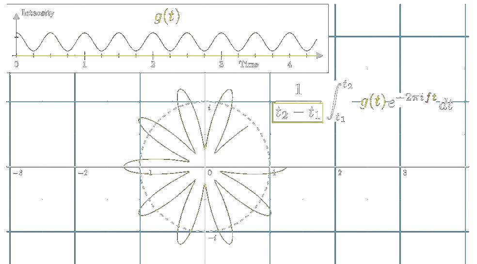
The Complex Fourier Transform

\(f(x)=a_0+\sum_{n=1}^\infty a_n\cos(nx)+\sum_{n=1}^\infty b_n\sin(nx)\)

\(\left\{\begin{array}{l}a_0=\frac1{2\pi}\int_{-\pi}^\pi f(x)\operatorname dx\\a_n=\frac1\pi\int_{-\pi}^\pi f(x)\cos(nx)\operatorname dx\\b_n=\frac1\pi\int_{-\pi}^\pi f(x)sin(nx)\operatorname dx\end{array}\right.\)

\(f(x)=\sum_{n=-\infty}^\infty c_ne^{inx}\)

\(c_n=\frac1{2\pi}\int_{-\pi}^\pi f(x)e^{-inx}dx\)

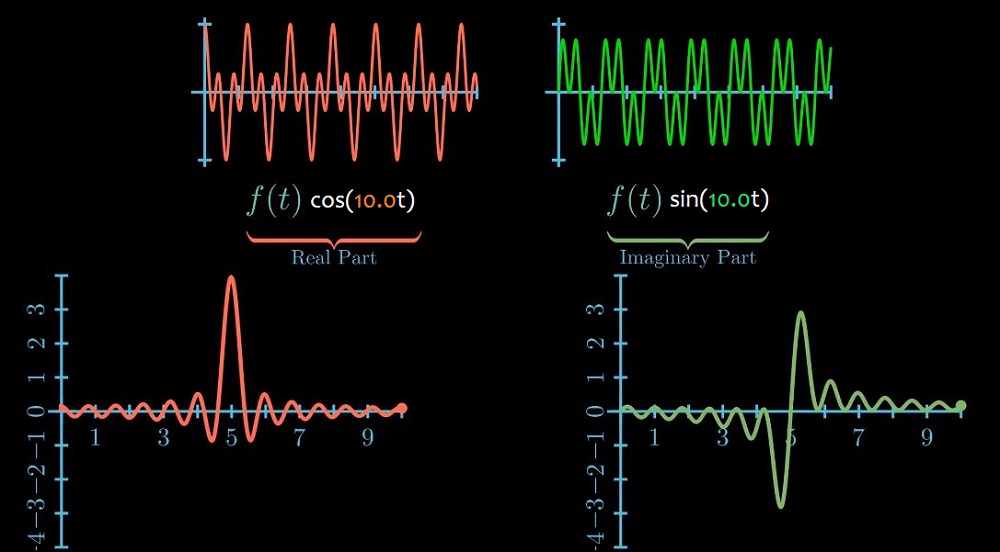
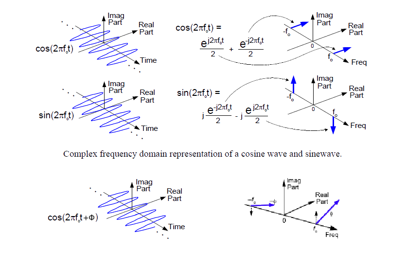
\(\left\{\begin{array}{l}\cos\theta=\frac{e^{i\theta}+e^{-i\theta}}2\\\sin\theta=\frac{e^{i\theta}-e^{-i\theta}}{2i}\end{array}\right.\)

\(f(x)=a_0+\sum_{n=1}^\infty a_n\cos(nx)+\sum_{n=1}^\infty b_n\sin(nx)\)
\(=a_0+\sum_{n=1}^\infty\frac{a_n}2(e^{inx}+e^{-inx})+\sum_{n=1}^\infty\frac{b_n}{2i}(e^{inx}-e^{-inx})\)
\(=\underbrace{a_0}_{c_0}+\sum_{n=1}^\infty\underbrace{(\frac{a_n-ib_n}2)}_{c_n}e^{inx}+\sum_{n=1}^\infty\underbrace{(\frac{a_n+ib_n}2)}_{c_{-n}}e^{-inx}\)
\(=c_0+\sum_{n=1}^\infty c_ne^{inx}+\sum_{n=1}^\infty c_{-n}e^{-inx}\)
\(=c_0+\sum_{n=1}^\infty c_ne^{inx}+\sum_{n=-1}^{-\infty}c_ne^{inx}\)
\(=\sum_{n=-\infty}^\infty c_ne^{inx}\)

\(\left\{\begin{array}{l}c_n=\frac{a_n-ib_n}2\\c_{-n}=\frac{a_n+ib_n}2\\c_0=a_0\end{array}\right.\;(n\geq1)\)

How to get \(c_n\)?

\(c_n=\frac{a_n-ib_n}2=\frac{{\displaystyle\frac1\pi}\int_{-\pi}^\pi f(x)\cos(nx)\operatorname dx-i\frac1\pi\int_{-\pi}^\pi f(x)\sin(nx)\operatorname dx}2\)
\(=\frac1{2\pi}\int_{-\pi}^\pi f(x)\cos(nx)\operatorname dx-i\frac1{2\pi}\int_{-\pi}^\pi f(x)\sin(nx)\operatorname dx\)
\(=\frac1{2\pi}\int_{-\pi}^\pi f(x)\lbrack\cos(nx)-i\sin(nx)\rbrack\operatorname dx\)

\(c_n=\frac1{2\pi}\int_{-\pi}^\pi f(x)e^{-inx}\operatorname dx\;(n\geq1)\)
\(c_{-n}=\frac1{2\pi}\int_{-\pi}^\pi f(x)e^{inx}\operatorname dx\;(n\geq1)\;\Rightarrow\;c_n=\frac1{2\pi}\int_{-\pi}^\pi f(x)e^{-inx}\operatorname dx\;(n\leq-1)\)
\(c_0=\frac1{2\pi}\int_{-\pi}^\pi f(x)\operatorname dx\)

\(\Rightarrow c_n=\frac1{2\pi}\int_{-\pi}^\pi f(x)e^{-inx}\operatorname dx,\;n\in\mathcal N\)

\(f(x)\in\mathcal Z\)

\(f(x)=g(x)+ih(x)\)
\(=\sum_{n=-\infty}^\infty g_ne^{inx}+i\sum_{n=-\infty}^\infty h_ne^{inx}\;(g_n,\;h_n\in\mathcal Z,\;(g_{-n},\;h_{-n})\;is\;the\;Complex\;conjugate\;of\;(g_n,\;h_n))\)
\(=\sum_{n=-\infty}^\infty\underbrace{(g_n+ih_n)}_{c_n}e^{inx}\)
\(c_n=g_n+ih_n\;\Rightarrow\;\overline{c_n}=\overline{g_n+ih_n}=\overline{g_n}-i\overline{h_n}=g_{-n}-ih_{-n}\)
\((c_{-n}=g_{-n}+ih_{-n})\neq\overline{c_n}\)

Complex Fourier Series

\(f(x)=\sum_{n=-\infty}^\infty c_ne^{inx}\)
\(c_n=\frac1{2\pi}\int_{-\pi}^\pi f(x)e^{-inx}\operatorname dx\)
\(\Rightarrow\int_{-\pi}^\pi e^{i(m-n)x}\operatorname dx=\left\{\begin{array}{lc}0&m\neq n\\2\pi&m=n\end{array}\right.\)

\(e^{inx}\rightarrow\left\{\begin{array}{lcc}n=0&f(x)=e^0=1&\\n=1&f(x)=e^{ix}&T=2\pi,\;\left\|f(x)\right\|=1\\n=2&f(x)=e^{i2x}&T=\pi,\;\left\|f(x)\right\|=1\\n=-1&f(x)=e^{-ix}&T=2\pi,\;\left\|f(x)\right\|=1\end{array}\right.\)

\(f(x)=\cdots+c_{-2}e^{-i2x}+c_{-1}e^{-ix}+c_0+c_1e^{ix}+c_2e^{i2x}+\cdots\)

The Orthogonality of Complex Basis

\(\cdots,e^{-i3x},e^{-i2x},e^{-ix},1,e^{ix},e^{i2x},e^{i3x},\cdots\)

\(\int_{-\pi}^\pi e^{imx}e^{inx}\operatorname dx\;\not>0\)

\(\int_{-\pi}^\pi e^{imx}e^{-inx}\operatorname dx=\int_{-\pi}^\pi e^{i(m-n)x}\operatorname dx=\left\{\begin{array}{lc}0&m\neq n\\2\pi&m=n\end{array}\right.\)

Standard basis for the field of complex numbers

\(\cdots,e^{-i3x},e^{-i2x},e^{-ix},1,e^{ix},e^{i2x},e^{i3x},\cdots\)

\(\int_{-\pi}^\pi e^{imx}e^{-inx}\operatorname dx=\left\{\begin{array}{lc}0&m\neq n\\2\pi&m=n\end{array}\right.,\;{\left\|e^{imx}\right\|}_C=\sqrt{2\pi}\)

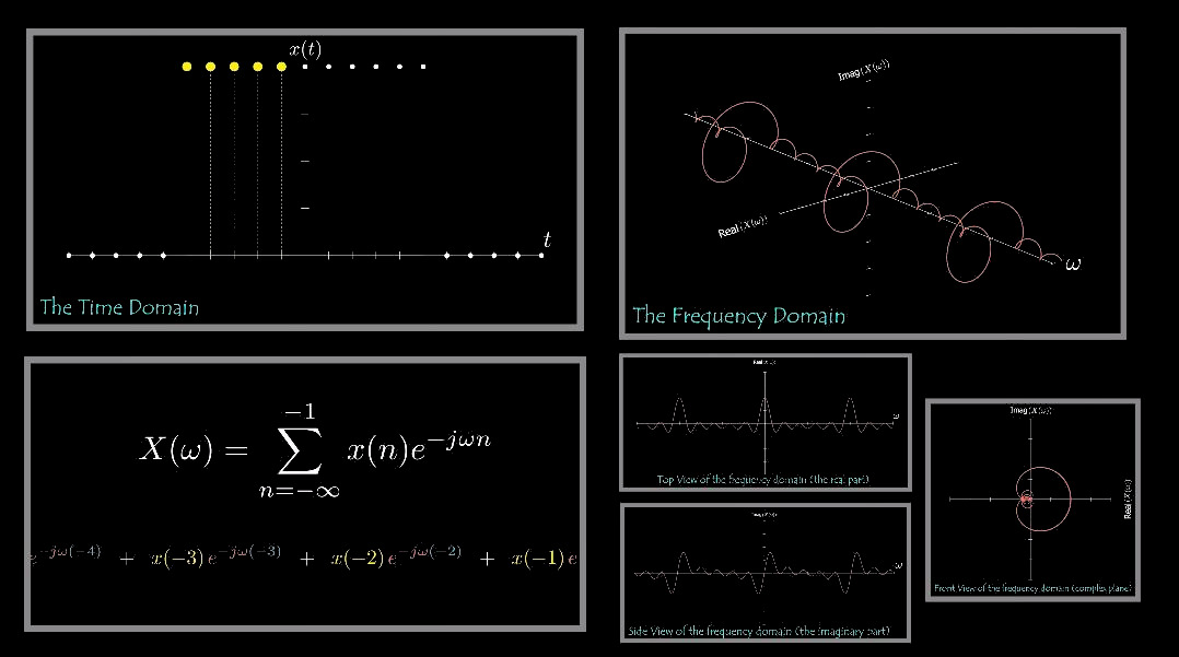
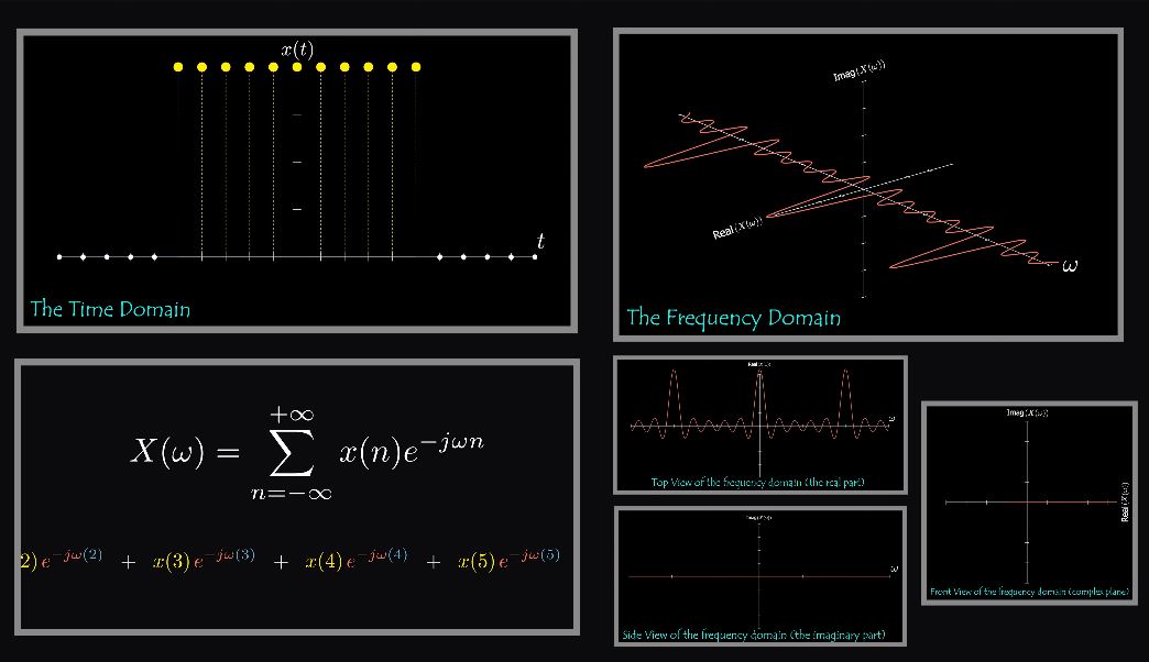
\(period:\;2\pi,\;f(x)=\sum_{n=-\infty}^\infty c_ne^{inx}\)

\(f(x)\;\xrightarrow{FT}\left[\cdots,c_{-k},c_{-k+1},\cdots,c_{-2},c_{-1},c_0,c_1,c_2,\cdots,c_{k-1},c_k,\cdots\right]\)

\(period:\;T,\;f(x)=\sum_{n=-\infty}^\infty c_ne^{\frac{i2\pi n}Tx}\)

\(f(x)\;\xrightarrow{FT}\left[\cdots,c_{-k},c_{-k+1},\cdots,c_{-2},c_{-1},c_0,c_1,c_2,\cdots,c_{k-1},c_k,\cdots\right]\)

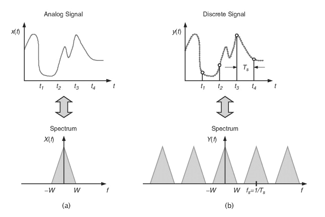
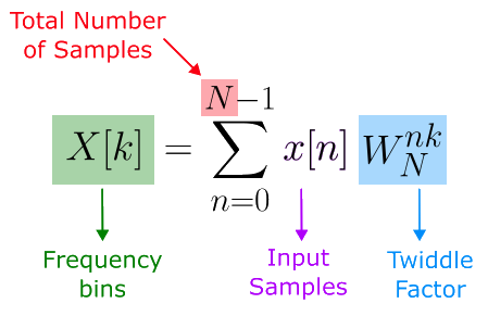
Discrete Fourier Transform

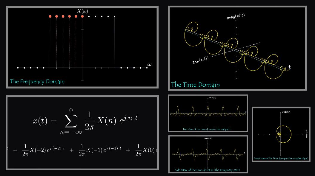
\(f(x)=\sum_{k=-\infty}^\infty c_ke^{ikx}\)

\(c_k=\frac1{2\pi}\int_{-\pi}^\pi f(x)e^{-ikx}\operatorname dx\)

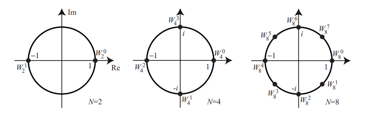
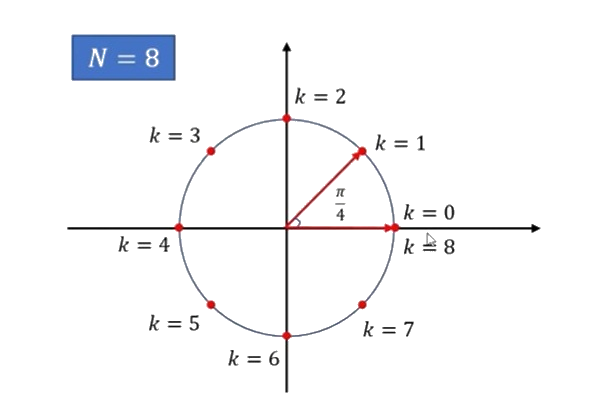
\(e^{k\frac{2\pi i}N},\;(k=0,1,\cdots,N-1)\)

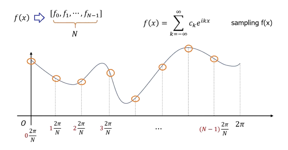
\(f(x)\) sampling

\(f(x)=\sum_{k=-\infty}^\infty c_ke^{ikx}\xrightarrow{x=\frac{2\pi}N}f_1=f(\frac{2\pi}N)=\sum_{k=-\infty}^\infty c_ke^{k\frac{2\pi i}N}\)

\(f(\frac{2\pi}N)=\cdots+c_{-2}e^{-2\cdot\frac{2\pi i}N}+c_{-1}e^{-1\cdot\frac{2\pi i}N}+c_0e^{0\cdot\frac{2\pi i}N}+c_1e^{1\cdot\frac{2\pi i}N}+c_2e^{2\cdot\frac{2\pi i}N}+\cdots+c_{k-1}e^{(k-1)\cdot\frac{2\pi i}N}+c_ke^{k\cdot\frac{2\pi i}N}+c_{k+1}e^{(k+1)\cdot\frac{2\pi i}N}+\cdots\)

\(what\;is\;e^{k\cdot\frac{2\pi i}N}?\)

\(f(\frac{2\pi}N)=\cdots+c_{-2}e^{-2\cdot\frac{2\pi i}N}+c_{-1}e^{-1\cdot\frac{2\pi i}N}+c_0e^{0\cdot\frac{2\pi i}N}+c_1e^{1\cdot\frac{2\pi i}N}+c_2e^{2\cdot\frac{2\pi i}N}+\cdots+c_{k-1}e^{(k-1)\cdot\frac{2\pi i}N}+c_ke^{k\cdot\frac{2\pi i}N}+c_{k+1}e^{(k+1)\cdot\frac{2\pi i}N}+\cdots\)
\(=(c_0+c_N+c_{-N}+c_{2N}+c_{-2N}+\cdots)e^{0\cdot\frac{2\pi i}N}\)
\(+(c_1+c_{N+1}+c_{-N+1}+c_{2N+1}+c_{-2N+1}+\cdots)e^{1\cdot\frac{2\pi i}N}\)
\(+(c_2+c_{N+2}+c_{-N+2}+c_{2N+2}+c_{-2N+2}+\cdots)e^{2\cdot\frac{2\pi i}N}\)
\(\dots\)
\(+(c_{N-1}+c_{2N-1}+c_{-1}+c_{3N-1}+c_{-N-1}+\cdots)e^{(N-1)\cdot\frac{2\pi i}N}\)

We don't need get infinite factors for each base. We could just keep one factor for each base.

\(f(\frac{2\pi}N)=\cdots+c_{-2}e^{-2\cdot\frac{2\pi i}N}+c_{-1}e^{-1\cdot\frac{2\pi i}N}+c_0e^{0\cdot\frac{2\pi i}N}+c_1e^{1\cdot\frac{2\pi i}N}+c_2e^{2\cdot\frac{2\pi i}N}+\cdots+c_{k-1}e^{(k-1)\cdot\frac{2\pi i}N}+c_ke^{k\cdot\frac{2\pi i}N}+c_{k+1}e^{(k+1)\cdot\frac{2\pi i}N}+\cdots\)
\(=(c_0+c_N+c_{-N}+c_{2N}+c_{-2N}+\cdots){\omega^0}\)
\(+(c_1+c_{N+1}+c_{-N+1}+c_{2N+1}+c_{-2N+1}+\cdots){\omega^1}\)
\(+(c_2+c_{N+2}+c_{-N+2}+c_{2N+2}+c_{-2N+2}+\cdots){\omega^2}\)
\(\dots\)
\(+(c_{N-1}+c_{2N-1}+c_{-1}+c_{3N-1}+c_{-N-1}+\cdots){\omega^{N-1}}\)

\(what\;is\;f(\frac{4\pi}N)?\)

\(f(2\cdot\frac{2\pi}N)=(c_0+c_N+c_{-N}+c_{2N}+c_{-2N}+\cdots){\omega^0}\)
\(+(c_1+c_{N+1}+c_{-N+1}+c_{2N+1}+c_{-2N+1}+\cdots){\omega^2}\)
\(+(c_2+c_{N+2}+c_{-N+2}+c_{2N+2}+c_{-2N+2}+\cdots){\omega^4}\)
\(\dots\)
\(+(c_{N-1}+c_{2N-1}+c_{-1}+c_{3N-1}+c_{-N-1}+\cdots){\omega^{2(N-1)}}\)

\(As\;\omega^N=1,\;for\;any\;k\in\mathcal Z,\;\omega^k\;will\;be\;one\;of\;\omega^0,\omega^1,\cdots,\omega^{N-1}\)

\(f(k\cdot\frac{2\pi}N)\;(k=0,1,\cdots,N-1)\;could\;be\;denoted\;by\;\omega^0,\omega^1,\cdots,\omega^{N-1}\)

If \(f(x)\) fourier series only contain \(c_0,c_1,c_2,\cdots,c_{N-1}\)

\(f(x)=c_0+c_1e^{ix}+c_2e^{i2x}+\cdots+c_{N-1}e^{i(N-1)x}\)

\(f(0\cdot\frac{2\pi}N)=c_0+c_1+c_2+\cdots+c_{N-1}\)
\(f(1\cdot\frac{2\pi}N)=c_0+c_1\omega+c_2\omega^2+\cdots+c_{N-1}\omega^{N-1}\)
\(f(2\cdot\frac{2\pi}N)=c_0+c_1\omega^2+c_2\omega^4+\cdots+c_{N-1}\omega^{2(N-1)}\)
\(f(3\cdot\frac{2\pi}N)=c_0+c_1\omega^3+c_2\omega^6+\cdots+c_{N-1}\omega^{3(N-1)}\)
\(\cdots\)
\(f((N-1)\cdot\frac{2\pi}N)=c_0+c_1\omega^{N-1}+c_2\omega^{2(N-1)}+\cdots+c_{N-1}\omega^{{(N-1)}^2}\)

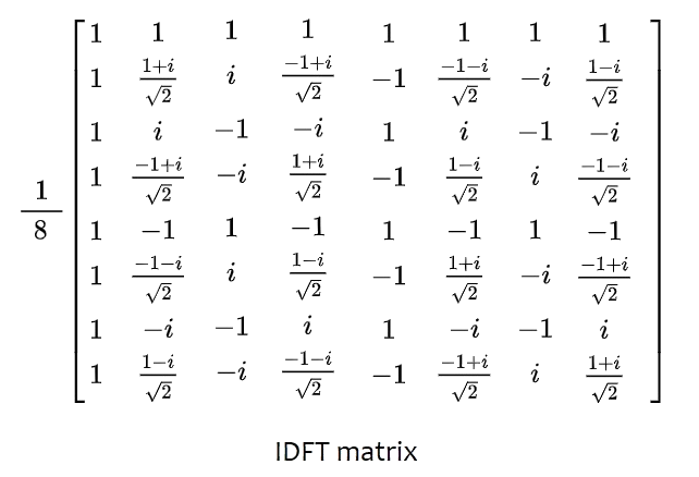
DFT matrix

\(\overbrace{\underset{\Leftarrow Inverse\;Discrete\;Fourier\;Transform}{\underbrace{\begin{bmatrix}f_0\\f_1\\f_2\\f_3\\\vdots\\f_{N-1}\end{bmatrix}\overset{DFT}{\underset{IDFT}\rightleftarrows}\begin{bmatrix}1&1&1&1&\cdots&1\\1&\omega&\omega^2&\omega^3&\cdots&\omega^{N-1}\\1&\omega^2&\omega^4&\omega^6&\cdots&\omega^{2(N-1)}\\1&\omega^3&\omega^6&\omega^9&\cdots&\omega^{3(N-1)}\\\vdots&\vdots&\vdots&\vdots&\ddots&\vdots\\1&\omega^{N-1}&\omega^{2(N-1)}&\omega^{3(N-1)}&\cdots&\omega^{{(N-1)}^2}\end{bmatrix}\begin{bmatrix}c_0\\c_1\\c_2\\c_3\\\vdots\\c_{N-1}\end{bmatrix}}}}^{\Rightarrow Discrete\;Fourier\;Transform}\)

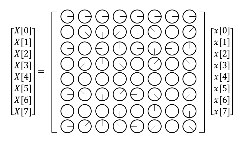
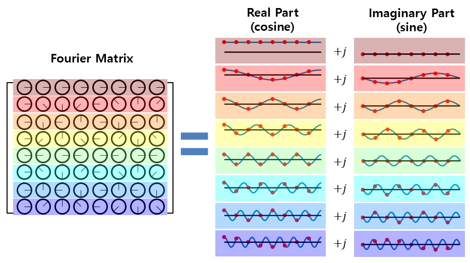
Fourier Matrix
\(\begin{bmatrix}1&1&1&1&\cdots&1\\1&\omega&\omega^2&\omega^3&\cdots&\omega^{N-1}\\1&\omega^2&\omega^4&\omega^6&\cdots&\omega^{2(N-1)}\\1&\omega^3&\omega^6&\omega^9&\cdots&\omega^{3(N-1)}\\\vdots&\vdots&\vdots&\vdots&\ddots&\vdots\\1&\omega^{N-1}&\omega^{2(N-1)}&\omega^{3(N-1)}&\cdots&\omega^{{(N-1)}^2}\end{bmatrix}\)

[Ex] \(f(x)=1+e^{ix}+e^{i2x}+e^{i3x}\)

N=4

\(f(0)=4,\;f(1\cdot\frac{2\pi}4)=f(2\cdot\frac{2\pi}4)=f(3\cdot\frac{2\pi}4)=0\)

\(\Rightarrow\omega=e^\frac{2\pi i}4=i\)

\(\begin{bmatrix}1&1&1&1\\1&\omega&\omega^2&\omega^3\\1&\omega^2&\omega^4&\omega^6\\1&\omega^3&\omega^6&\omega^9\end{bmatrix}^{-1}\begin{bmatrix}4\\0\\0\\0\end{bmatrix}=\begin{bmatrix}1\\1\\1\\1\end{bmatrix}\)

N=3

\(f(0)=4,\;f(\frac{2\pi}3)=1,\;f(2\cdot\frac{2\pi}3)=1\)

\(\omega=e^\frac{2\pi i}3=-\frac12+\frac{\sqrt3}2i\)

\(\begin{bmatrix}1&1&1\\1&\omega&\omega^2\\1&\omega^2&\omega^4\end{bmatrix}^{-1}\begin{bmatrix}4\\1\\1\end{bmatrix}=\begin{bmatrix}2\\1\\1\end{bmatrix}\)

\(\begin{bmatrix}{\color[rgb]{0.0, 0.0, 1.0}2}\\1\\1\end{bmatrix}\Rightarrow{\color[rgb]{0.0, 0.0, 1.0}2}\;is\;{\color[rgb]{0.0, 0.0, 1.0}1}+e^{ix}+e^{i2x}+{\color[rgb]{0.0, 0.0, 1.0}1}\cdot e^{i3x},\;({\color[rgb]{1.0, 0.0, 0.0}1}\cdot e^{-ix}+{\color[rgb]{1.0, 0.0, 0.0}1}+e^{ix}+e^{i2x})\;\begin{bmatrix}{\color[rgb]{1.0, 0.0, 0.0}1}\\1\\1\\{\color[rgb]{0.68, 0.46, 0.12}1}\end{bmatrix}\)

N=6

\(f(0)=4,\;f(1\cdot\frac{2\pi}6)=\sqrt3i,\;f(2\cdot\frac{2\pi}6)=1\)
\(f(3\cdot\frac{2\pi}6)=0,\;f(4\cdot\frac{2\pi}6)=1,\;f(5\cdot\frac{2\pi}6)=-\sqrt3i\)

\(\omega=e^\frac{2\pi i}6=\frac12+\frac{\sqrt3}2i\)

\(\omega_6^{-1}\begin{bmatrix}4\\\sqrt3i\\1\\0\\1\\-\sqrt3i\end{bmatrix}=\begin{bmatrix}1\\1\\1\\1\\0\\0\end{bmatrix}\)

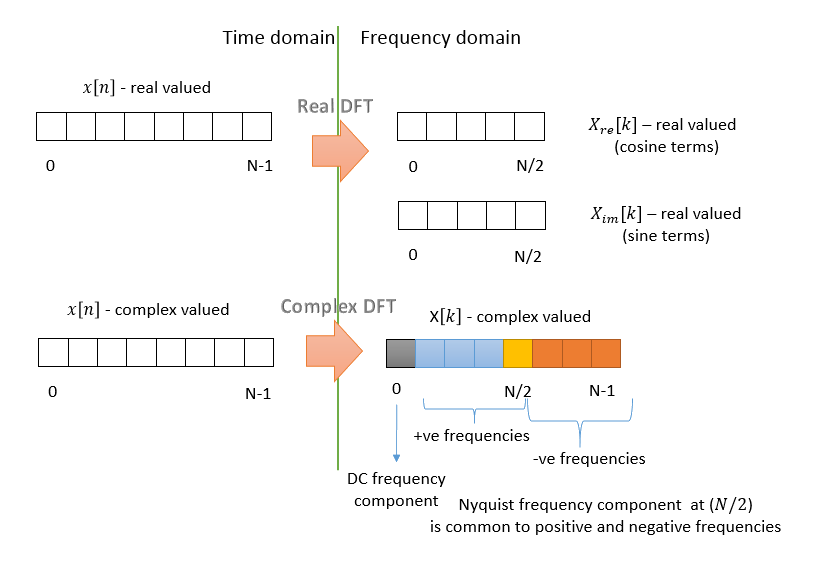
DFT for Real number function

[Ex] \(f(x)=1+\cos(x)+\cos(2x)\)

\(f(x)=\frac12e^{-i2x}+\frac12e^{-ix}+1+\frac12e^{ix}+\frac12e^{i2x}\)

N=6

\(\omega_6^{-1}\begin{bmatrix}3\\1\\0\\1\\0\\1\end{bmatrix}=\begin{bmatrix}1\\0.5\\0.5\\0\\0.5\\0.5\end{bmatrix}\Rightarrow\begin{bmatrix}{\color[rgb]{0.0, 0.0, 1.0}1}&\frac12e^{-i2x}+\frac12e^{-ix}+\boxed{\color[rgb]{0.0, 0.0, 1.0}1}+\frac12e^{ix}+\frac12e^{i2x}\\{\color[rgb]{1.0, 0.0, 1.0}0}{\color[rgb]{1.0, 0.0, 1.0}.}{\color[rgb]{1.0, 0.0, 1.0}5}&\frac12e^{-i2x}+\frac12e^{-ix}+1+\boxed{{\color[rgb]{1.0, 0.0, 1.0}\frac12}e^{ix}}+\frac12e^{i2x}\\{\color[rgb]{0.9, 0.76, 0.02}0}{\color[rgb]{0.9, 0.76, 0.02}.}{\color[rgb]{0.9, 0.76, 0.02}5}&\frac12e^{-i2x}+\frac12e^{-ix}+1+\frac12e^{ix}+\boxed{{\color[rgb]{0.9, 0.76, 0.02}\frac12}e^{i2x}}\\0&\frac12e^{-i2x}+\frac12e^{-ix}+1+\frac12e^{ix}+\frac12e^{i2x}\\{\color[rgb]{0.0, 0.0, 1.0}0}{\color[rgb]{0.0, 0.0, 1.0}.}{\color[rgb]{0.0, 0.0, 1.0}5}&\boxed{{\color[rgb]{0.0, 0.0, 1.0}\frac12}e^{-i2x}}+\frac12e^{-ix}+1+\frac12e^{ix}+\frac12e^{i2x}\\{\color[rgb]{0.0, 0.0, 0.5}0}{\color[rgb]{0.0, 0.0, 0.5}.}{\color[rgb]{0.0, 0.0, 0.5}5}&\frac12e^{-i2x}+\boxed{{\color[rgb]{0.0, 0.0, 0.5}\frac12}e^{-ix}}+1+\frac12e^{ix}+\frac12e^{i2x}\end{bmatrix}\)

N=4

\(\omega_4^{-1}\begin{bmatrix}3\\0\\1\\0\end{bmatrix}=\begin{bmatrix}1\\0.5\\1\\0.5\end{bmatrix}\Rightarrow\begin{bmatrix}{\color[rgb]{0.0, 0.0, 1.0}1}&\frac12e^{-i2x}+\frac12e^{-ix}+\boxed{\color[rgb]{0.0, 0.0, 1.0}1}+\frac12e^{ix}+\frac12e^{i2x}\\{\color[rgb]{0.9, 0.76, 0.02}0}{\color[rgb]{0.9, 0.76, 0.02}.}{\color[rgb]{0.9, 0.76, 0.02}5}&\frac12e^{-i2x}+\frac12e^{-ix}+1+\boxed{{\color[rgb]{0.9, 0.76, 0.02}\frac12}e^{ix}}+\frac12e^{i2x}\\{\color[rgb]{1.0, 0.0, 1.0}1}&\boxed{{\color[rgb]{1.0, 0.0, 1.0}\frac12}e^{-i2x}}+\frac12e^{-ix}+1+\frac12e^{ix}+\boxed{{\color[rgb]{1.0, 0.0, 1.0}\frac12}e^{i2x}}\\{\color[rgb]{0.0, 0.5, 0.5}0}{\color[rgb]{0.0, 0.5, 0.5}.}{\color[rgb]{0.0, 0.5, 0.5}5}&\frac12e^{-i2x}+\boxed{{\color[rgb]{0.0, 0.5, 0.5}\frac12}e^{-ix}}+1+\frac12e^{ix}+\frac12e^{i2x}\end{bmatrix}\)

N=5

\(\omega_5^{-1}\begin{bmatrix}3\\0.5\\0.5\\0.5\\0.5\end{bmatrix}=\begin{bmatrix}1\\0.5\\0.5\\0.5\\0.5\end{bmatrix}=\begin{bmatrix}1&\frac12e^{-i2x}+\frac12e^{-ix}+\boxed1+\frac12e^{ix}+\frac12e^{i2x}\\0.5&\frac12e^{-i2x}+\frac12e^{-ix}+1+\boxed{\frac12e^{ix}}+\frac12e^{i2x}\\0.5&\frac12e^{-i2x}+\frac12e^{-ix}+1+\frac12e^{ix}+\boxed{\frac12e^{i2x}}\\0.5&\boxed{\frac12e^{-i2x}}+\frac12e^{-ix}+1+\frac12e^{ix}+\frac12e^{i2x}\\0.5&\frac12e^{-i2x}+\boxed{\frac12e^{-ix}}+1+\frac12e^{ix}+\frac12e^{i2x}\end{bmatrix}\)

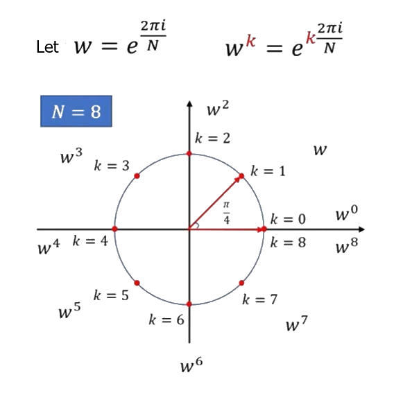
\(\omega=e^\frac{2\pi i}N\Rightarrow\omega^k=e^{k\cdot\frac{2\pi i}N}\)

Characteristics of DFT

IDFT

\(\begin{bmatrix}f_0\\f_1\\f_2\\f_3\\\vdots\\f_k\\\vdots\\f_{N-1}\end{bmatrix}=\begin{bmatrix}1&1&1&1&\dots&1\\1&\omega&\omega^2&\omega^3&\dots&\omega^{N-1}\\1&\omega^2&\omega^4&\omega^6&\dots&\omega^{2(N-1)}\\1&\omega^3&\omega^6&\omega^9&\dots&\omega^{3(N-1)}\\\vdots&\vdots&\vdots&\vdots&\vdots&\vdots\\1&\omega^k&(\omega^k)^2&(\omega^k)^3&\dots&\omega^{k(N-1)}\\\vdots&\vdots&\vdots&\vdots&\vdots&\vdots\\1&\omega^{N-1}&\omega^{2(N-1)}&\omega^{3(N-1)}&\dots&\omega^{(N-1)(N-1)}\end{bmatrix}\begin{bmatrix}c_0\\c_1\\c_2\\c_3\\\vdots\\c_k\\\vdots\\c_{N-1}\end{bmatrix}\)

\(\omega=e^\frac{2\pi i}N\)

\(F_NF_N^\ast=N\begin{bmatrix}1&0&0\\0&\ddots&0\\0&0&1\end{bmatrix}\Rightarrow F_N^{-1}=\frac1NF_N^\ast\)

DFT

\(\frac1N\begin{bmatrix}1&1&1&1&\dots&1\\1&\overline\omega&\overline\omega^2&\overline\omega^3&\dots&\overline\omega^{N-1}\\1&\overline\omega^2&\overline\omega^4&\overline\omega^6&\dots&\overline\omega^{2(N-1)}\\1&\overline\omega^3&\overline\omega^6&\overline\omega^9&\dots&\overline\omega^{3(N-1)}\\\vdots&\vdots&\vdots&\vdots&\vdots&\vdots\\1&\overline\omega^k&(\overline\omega^k)^2&(\overline\omega^k)^3&\dots&\overline\omega^{k(N-1)}\\\vdots&\vdots&\vdots&\vdots&\vdots&\vdots\\1&\overline\omega^{N-1}&\overline\omega^{2(N-1)}&\overline\omega^{3(N-1)}&\dots&\overline\omega^{(N-1)(N-1)}\end{bmatrix}\begin{bmatrix}f_0\\f_1\\f_2\\f_3\\\vdots\\f_k\\\vdots\\f_{N-1}\end{bmatrix}=\begin{bmatrix}c_0\\c_1\\c_2\\c_3\\\vdots\\c_k\\\vdots\\c_{N-1}\end{bmatrix}\)

\(\overline\omega=e^{-\frac{2\pi i}N}\)

a useful property:
\(\begin{array}{rcl}\omega^0+\omega^1+\dots+\omega^{N-1}&{}={}&\frac{1-\omega^N}{1-\omega}\\&{}={}&\frac{1-1}{1-\omega}\\&{}={}&0\end{array}\)

Now consider the inner product between any two rows other than the first, say row \(p\) and row \(q\)

\(\left\langle row_p\vert row_q\right\rangle=1+(\omega^p)^\ast(\omega^q)+(\omega^{2p})^\ast(\omega^{2q})+\dots+(\omega^{p(N-1)})^\ast(\omega^{q(N-1)})\), Remember left-side conjugation
\(=1+\omega^{-p}\omega^q+\omega^{-2p}\omega^{2q}+\dots+\omega^{-p(N-1)}\omega^{q(N-1)}\), \({(\omega^k)}^\ast=\omega^{-k}\)
\(=1+\omega^{q-p}+(\omega^{q-p})^2+\dots+(\omega^{q-p})^{(N-1)}\), Exponent algebra
\(=\frac{1-(\omega^{q-p})^N}{1-\omega^{q-p}}\), Geometric series
\(=\frac{1-(\omega^N)^{q-p}}{1-\omega^{q-p}}\), Exponent algebra
\(=\frac{1-(1)^{q-p}}{1-\omega^{q-p}}\), \(\omega\) is an \(N_{th}\) root
\(=0\)

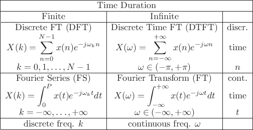
The DFT

\(\widetilde v=Dv\)

\(\begin{bmatrix}{\widetilde a}_0\\{\widetilde a}_1\\{\widetilde a}_2\\\vdots\\{\widetilde a}_{N-1}\end{bmatrix}{}={}\begin{bmatrix}1&1&1&\dots&1\\(\omega)^0&\omega&\omega^2&\dots&\omega^{N-1}\\(\omega^2)^0&\omega^2&\omega^4&\dots&\omega^{2(N-1)}\\(\omega^3)^0&\omega^3&\omega^6&\dots&\omega^{3(N-1)}\\\vdots&\vdots&\vdots&\vdots&\vdots\\(\omega^k)^0&\omega^k&(\omega^k)^2&\dots&\omega^{k(N-1)}\\\vdots&\vdots&\vdots&\vdots&\vdots\\(\omega^{N-1})^0&\omega^{N-1}&\omega^{2(N-1)}&\dots&\omega^{(N-1)(N-1)}\end{bmatrix}{}\begin{bmatrix}a_0\\a_1\\a_2\\\vdots\\a_{N-1}\end{bmatrix}\)

\(v=D^{-1}\widetilde v=\frac1ND^\dagger\widetilde v\)

\(\overline v=D^\dagger v\)

\(D^\dagger=the\;Discreate\;Fourier\;Transform\)

\((D^\dagger)^{-1}=\frac1ND=Inverse\;DFT\)

The unitary DFT

Because \(D^\dagger D = NI \neq I\), , the matrix \(D\) is not unitary.

This is rather simple to fix. Define
\(U_{DFT}=\frac1{\sqrt N}D\)
\(U_{DFT}^\dagger=\frac1{\sqrt N}D^\dagger\)
\(U_{DFT}^\dagger U_{DFT}=\frac1{\sqrt N}D^\dagger\frac1{\sqrt N}D=I\)

[Ex] \(\begin{bmatrix}4\\0\\0\\0\end{bmatrix},\;\omega=e^\frac{2\pi i}4=i,\;f(x)=\left\{\begin{array}{l}f(0\cdot\frac{2\pi}4)=4\\f(1\cdot\frac{2\pi}4)=0\\f(2\cdot\frac{2\pi}4)=0\\f(3\cdot\frac{2\pi}4)=0\end{array}\right.\)

\(f(x)=\sum_{k=-\infty}^\infty c_ke^{ikx}\)

\(f(0\cdot\frac{2\pi}4)\Rightarrow\left\{\begin{array}{l}=(\cdots+c_{-4}+c_0+c_4+\cdots)\omega^0\\+(\cdots+c_{-3}+c_1+c_5+\cdots)\omega^0\\+(\cdots+c_{-2}+c_2+c_6+\cdots)\omega^0\\+(\cdots+c_{-1}+c_3+c_7+\cdots)\omega^0\end{array}\right.\)

\(f(1\cdot\frac{2\pi}4)\Rightarrow\left\{\begin{array}{l}=(\cdots+c_{-4}+c_0+c_4+\cdots)\omega^0\\+(\cdots+c_{-3}+c_1+c_5+\cdots)\omega^1\\+(\cdots+c_{-2}+c_2+c_6+\cdots)\omega^2\\+(\cdots+c_{-1}+c_3+c_7+\cdots)\omega^3\end{array}\right.\)

\(f(2\cdot\frac{2\pi}4)\Rightarrow\left\{\begin{array}{l}=(\cdots+c_{-4}+c_0+c_4+\cdots)\omega^0\\+(\cdots+c_{-3}+c_1+c_5+\cdots)\omega^2\\+(\cdots+c_{-2}+c_2+c_6+\cdots)\omega^4\\+(\cdots+c_{-1}+c_3+c_7+\cdots)\omega^6\end{array}\right.\)

\(f(3\cdot\frac{2\pi}4)\Rightarrow\left\{\begin{array}{l}=(\cdots+c_{-4}+c_0+c_4+\cdots)\omega^0\\+(\cdots+c_{-3}+c_1+c_5+\cdots)\omega^3\\+(\cdots+c_{-2}+c_2+c_6+\cdots)\omega^6\\+(\cdots+c_{-1}+c_3+c_7+\cdots)\omega^9\end{array}\right.\)

\(\begin{bmatrix}f(0\cdot\frac{2\pi}4)\\f(1\cdot\frac{2\pi}4)\\f(2\cdot\frac{2\pi}4)\\f(3\cdot\frac{2\pi}4)\end{bmatrix}=\begin{bmatrix}1&1&1&1\\1&\omega&\omega^2&\omega^3\\1&\omega^2&\omega^4&\omega^6\\1&\omega^3&\omega^6&\omega^9\end{bmatrix}\begin{bmatrix}(\cdots+c_{-4}+c_0+c_4+\cdots)\\(\cdots+c_{-3}+c_1+c_5+\cdots)\\(\cdots+c_{-2}+c_2+c_6+\cdots)\\(\cdots+c_{-1}+c_3+c_7+\cdots)\end{bmatrix}\)

\(f(x)=1+e^{ix}+e^{i2x}+e^{i3x}\)

\(f(x)=1+e^{ix}+e^{i2x}+e^{-ix}\)

\(f(x)=\frac12e^{-ix}+1+e^{ix}+e^{i2x}+\frac12e^{i3x}\)

\(f(x)=1+\frac13e^{ix}+\frac13e^{i5x}+\frac13e^{i9x}+e^{i2x}+e^{i3x}\\f(x)=\frac12e^{-ix}+1+e^{ix}+e^{i2x}+\frac12e^{i3x}\)

\(f(x)=e^{ix}+e^{i2x}+e^{i3x}+e^{i4x}\)

Fourier Series

Expand \(f(x)\) by using the orthogonal set of trigonometric functions
\[f(x)=\frac{a_0}2+\sum_{n=1}^\infty(a_n\cos\frac{n\pi}px+b_n\sin\frac{n\pi}px)\]

Coefficients of each orthogonal function can be determined by inner product from \(-p\) to \(p\).

(i) coef. of \(1\): \(\int_{-p}^pf(x)\cdot1\operatorname dx=\int_{-p}^p\lbrack\frac{a_0}2+\sum_{n=1}^\infty(a_n\underbrace{\cos\frac{n\pi}px}_\cancel{\sin\frac{n\pi}px}+b_n\underbrace{\sin\frac{n\pi}px}_\cancel{-\cos\frac{n\pi}px})\rbrack dx=\frac{a_0}2\int_{-p}^pdx=a_0\cdot p\)

\(\therefore a_0=\frac1p\int_{-p}^pf(x)\operatorname dx\)

\(\Rightarrow c_n={\left.\frac{\left\langle f(x),\phi_n(x)\right\rangle}{\left\langle\phi_n(x),\phi_n(x)\right\rangle}\right|}_{\phi_n=1}=\frac{\int_{-p}^pf(x)\operatorname dx}{\int_{-p}^p1^2\operatorname dx}=\frac{a_0\cdot p}{2p}=\frac{a_0}2\)

(ii) coef. of \(\cos\frac{m\pi}px\): \(\int_{-p}^pf(x)\cdot\cos\frac{m\pi}px\operatorname dx=\int_{-p}^p\lbrack\underbrace{\frac{a_0}2\cdot\cos\frac{m\pi}px}_{=0}+\sum_{n=1}^\infty(a_n\underbrace{\cos\frac{m\pi}px\cdot\cos\frac{n\pi}px}_{\frac12\lbrack\cos\frac{(m+n)\pi}px+\cos\frac{(m-n)\pi}px\rbrack}+b_n\underbrace{\cos\frac{m\pi}px\cdot\sin\frac{n\pi}px}_{\frac12\lbrack\sin\frac{(m+n)\pi}px+\sin\frac{(m-n)\pi}px\rbrack=0})\rbrack dx\)

\(\int_{-p}^p\frac12\lbrack\cos\frac{(m+n)\pi}px+\cos\frac{(m-n)\pi}px\rbrack dx=\left\{\begin{array}{lc}0&m\neq n\\p&m=n\end{array}\right.\)

\(m=n,\;\int_{-p}^p{(\cos\frac{m\pi}px)}^2dx=\int_{-p}^p\frac{1+\cancel{\cos\frac{2m\pi}px}}2dx=p\)

(iiI) coef. of \(\sin\frac{m\pi}px\): \(\int_{-p}^pf(x)\cdot\sin\frac{m\pi}px\operatorname dx=\int_{-p}^p\lbrack\underbrace{\frac{a_0}2\cdot\sin\frac{m\pi}px}_{=0}+\sum_{n=1}^\infty(a_n\underbrace{\cos\frac{m\pi}px\cdot\sin\frac{n\pi}px}_{\frac12\lbrack\sin\frac{(m+n)\pi}px+\sin\frac{(m-n)\pi}px\rbrack=0}+b_n\underbrace{\sin\frac{m\pi}px\cdot\sin\frac{n\pi}px}_{\frac12\lbrack\cos\frac{(m-n)\pi}px-\sin\frac{(m+n)\pi}px\rbrack})\rbrack dx\)

\(\int_{-p}^p\frac12\lbrack\cos\frac{(m-n)\pi}px-\sin\frac{(m+n)\pi}px\rbrack dx=\left\{\begin{array}{l}0,\;m\neq n\\p,\;m=n\end{array}\right.\)

\(m=n,\;\int_{-p}^p{(\sin\frac{m\pi}px)}^2dx=\int_{-p}^p\frac{1-\cancel{\cos\frac{2m\pi}px}}2dx=p\)

\(\Rightarrow\left\{\begin{array}{l}a_n=\frac1p\int_{-p}^pf(x)\cdot\cos\frac{n\pi}px\operatorname dx\\b_n=\frac1p\int_{-p}^pf(x)\cdot\sin\frac{n\pi}px\operatorname dx\end{array}\right.\)

The Fourier series of a function \(f\) defined on the internal \([-p,p]\) is given by
\(f(x)=\frac{a_0}2+\sum_{n=1}^\infty(a_n\cos\frac{n\pi}px+b_n\sin\frac{n\pi}px)\)
where \(\left\{\begin{array}{l}a_0=\frac1p\int_{-p}^pf(x)\operatorname dx\\a_n=\frac1p\int_{-p}^pf(x)\cdot\cos\frac{n\pi}px\operatorname dx\\b_n=\frac1p\int_{-p}^pf(x)\cdot\sin\frac{n\pi}px\operatorname dx\end{array}\right.\)

\(f\): odd function \(\Rightarrow f(-x)=-f(x)\)

\(f\): even function \(\Rightarrow f(-x)=f(x)\)

Fourier cosine and sine series

For an even function \(f\) defined on the interval \([-p,p]\), the Fourier series is the Fourier cosine series:

\(f(x)=\frac{a_0}2+\sum_{n=1}^\infty a_n\cos\frac{n\pi}px\)

where \(\left\{\begin{array}{l}a_0=\frac1p\int_{-p}^pf(x)\operatorname dx\\a_n=\frac2p\int_0^pf(x)\cdot\cos\frac{n\pi}px\operatorname dx\end{array}\right.\)

For an odd function \(f\) defined on the interval \([-p,p]\), the Fourier series is the Fourier sine series:

\(f(x)=\sum_{n=1}^\infty b_n\sin\frac{n\pi}px\)

where \(b_n=\frac2p\int_0^pf(x)\cdot\sin\frac{n\pi}px\operatorname dx\)

Fast Fourier Transform (FFT)

\(\begin{bmatrix}1&1&1&1&\dots&1\\1&\overline\omega&\overline\omega^2&\overline\omega^3&\dots&\overline\omega^{N-1}\\1&\overline\omega^2&\overline\omega^4&\overline\omega^6&\dots&\overline\omega^{2(N-1)}\\1&\overline\omega^3&\overline\omega^6&\overline\omega^9&\dots&\overline\omega^{3(N-1)}\\\vdots&\vdots&\vdots&\vdots&\vdots&\vdots\\1&\overline\omega^k&(\overline\omega^k)^2&(\overline\omega^k)^3&\dots&\overline\omega^{k(N-1)}\\\vdots&\vdots&\vdots&\vdots&\vdots&\vdots\\1&\overline\omega^{N-1}&\overline\omega^{2(N-1)}&\overline\omega^{3(N-1)}&\dots&\overline\omega^{(N-1)(N-1)}\end{bmatrix}\begin{bmatrix}f_0\\f_1\\f_2\\f_3\\\vdots\\f_k\\\vdots\\f_{N-1}\end{bmatrix}\)

\(\begin{bmatrix}{\overline x}_1&{\color[rgb]{0.0, 0.0, 1.0}\overline x}_{\color[rgb]{0.0, 0.0, 1.0}2}&{\overline x}_3&{\color[rgb]{0.9, 0.76, 0.02}\overline x}_{\color[rgb]{0.9, 0.76, 0.02}4}\end{bmatrix}\begin{bmatrix}a_1\\{\color[rgb]{0.0, 0.0, 1.0}a}_{\color[rgb]{0.0, 0.0, 1.0}2}\\a_3\\{\color[rgb]{0.9, 0.76, 0.02}a}_{\color[rgb]{0.9, 0.76, 0.02}4}\end{bmatrix}=a_1{\overline x}_1+{\color[rgb]{0.0, 0.0, 1.0}a}_{\color[rgb]{0.0, 0.0, 1.0}2}{\color[rgb]{0.0, 0.0, 1.0}\overline x}_{\color[rgb]{0.0, 0.0, 1.0}2}+a_3{\overline x}_3+{\color[rgb]{0.9, 0.76, 0.02}a}_{\color[rgb]{0.9, 0.76, 0.02}4}{\color[rgb]{0.9, 0.76, 0.02}\overline x}_{\color[rgb]{0.9, 0.76, 0.02}4}\)

\(\begin{bmatrix}{\overline x}_1&{\color[rgb]{0.9, 0.76, 0.02}\overline x}_{\color[rgb]{0.9, 0.76, 0.02}4}&{\overline x}_3&{\color[rgb]{0.0, 0.0, 1.0}\overline x}_{\color[rgb]{0.0, 0.0, 1.0}2}\end{bmatrix}\begin{bmatrix}a_1\\{\color[rgb]{0.9, 0.76, 0.02}a}_{\color[rgb]{0.9, 0.76, 0.02}4}\\a_3\\{\color[rgb]{0.0, 0.0, 1.0}a}_{\color[rgb]{0.0, 0.0, 1.0}2}\end{bmatrix}=a_1{\overline x}_1+{\color[rgb]{0.9, 0.76, 0.02}a}_{\color[rgb]{0.9, 0.76, 0.02}4}{\color[rgb]{0.9, 0.76, 0.02}\overline x}_{\color[rgb]{0.9, 0.76, 0.02}4}+a_3{\overline x}_3+{\color[rgb]{0.0, 0.0, 1.0}a}_{\color[rgb]{0.0, 0.0, 1.0}2}{\color[rgb]{0.0, 0.0, 1.0}\overline x}_{\color[rgb]{0.0, 0.0, 1.0}2}\)

To swap items of row and column accordingly of matrix multiplication is able to keep the ordinary result.

\(F_4=\begin{bmatrix}1&1&1&1\\1&\overline\omega^1&\overline\omega^2&\overline\omega^3\\1&\overline\omega^2&\overline\omega^4&\overline\omega^6\\1&\overline\omega^3&\overline\omega^6&\overline\omega^9\end{bmatrix}\begin{bmatrix}f_0\\f_1\\f_2\\f_3\end{bmatrix}\)

\(\Rightarrow{\widetilde F}_4=\begin{bmatrix}1&1&1&1\\1&\overline\omega^2&\overline\omega^1&\overline\omega^3\\1&\overline\omega^4&\overline\omega^2&\overline\omega^6\\1&\overline\omega^6&\overline\omega^3&\overline\omega^9\end{bmatrix}\begin{bmatrix}f_0\\f_2\\f_1\\f_3\end{bmatrix}\)

\(\begin{bmatrix}1&1&1&1\\1&\overline\omega^1&\overline\omega^2&\overline\omega^3\\1&\overline\omega^2&\overline\omega^4&\overline\omega^6\\1&\overline\omega^3&\overline\omega^6&\overline\omega^9\end{bmatrix}\Rightarrow\begin{bmatrix}1&1&1&1\\1&\overline\omega^2&\overline\omega^1&\overline\omega^3\\1&\overline\omega^4&\overline\omega^2&\overline\omega^6\\1&\overline\omega^6&\overline\omega^3&\overline\omega^9\end{bmatrix}\)

\(\begin{bmatrix}{\color[rgb]{0.0, 0.0, 1.0}1}&{\color[rgb]{0.0, 0.0, 1.0}1}&{\color[rgb]{0.51, 0.5, 0.0}1}&{\color[rgb]{0.51, 0.5, 0.0}1}\\{\color[rgb]{0.0, 0.0, 1.0}1}&\color[rgb]{0.0, 0.0, 1.0}\overline\omega^2&\color[rgb]{0.51, 0.5, 0.0}\overline\omega^1&\color[rgb]{0.51, 0.5, 0.0}\overline\omega^3\\{\color[rgb]{0.9, 0.76, 0.02}1}&\color[rgb]{0.9, 0.76, 0.02}\overline\omega^4&\color[rgb]{0.7, 0.7, 0.7}\overline\omega^2&\color[rgb]{0.7, 0.7, 0.7}\overline\omega^6\\{\color[rgb]{0.9, 0.76, 0.02}1}&\color[rgb]{0.9, 0.76, 0.02}\overline\omega^6&\color[rgb]{0.7, 0.7, 0.7}\overline\omega^3&\color[rgb]{0.7, 0.7, 0.7}\overline\omega^9\end{bmatrix}\Rightarrow F_2=\begin{bmatrix}{\color[rgb]{0.0, 0.0, 1.0}1}&{\color[rgb]{0.0, 0.0, 1.0}1}\\{\color[rgb]{0.0, 0.0, 1.0}1}&\color[rgb]{0.0, 0.0, 1.0}\overline\omega^2\end{bmatrix},\;F_2=\begin{bmatrix}{\color[rgb]{0.9, 0.76, 0.02}1}&\color[rgb]{0.9, 0.76, 0.02}\overline\omega^4\\{\color[rgb]{0.9, 0.76, 0.02}1}&\color[rgb]{0.9, 0.76, 0.02}\overline\omega^6\end{bmatrix}=\begin{bmatrix}{\color[rgb]{0.0, 0.0, 1.0}1}&{\color[rgb]{0.0, 0.0, 1.0}1}\\{\color[rgb]{0.0, 0.0, 1.0}1}&\color[rgb]{0.0, 0.0, 1.0}\overline\omega^2\end{bmatrix}\)

\(\Rightarrow\begin{bmatrix}{\color[rgb]{0.51, 0.5, 0.0}1}&{\color[rgb]{0.51, 0.5, 0.0}1}\\\color[rgb]{0.51, 0.5, 0.0}\overline\omega^1&\color[rgb]{0.51, 0.5, 0.0}\overline\omega^3\end{bmatrix}=\begin{bmatrix}1&0\\0&\overline\omega\end{bmatrix}F_2,\;\begin{bmatrix}\color[rgb]{0.7, 0.7, 0.7}\overline\omega^2&\color[rgb]{0.7, 0.7, 0.7}\overline\omega^6\\\color[rgb]{0.7, 0.7, 0.7}\overline\omega^3&\color[rgb]{0.7, 0.7, 0.7}\overline\omega^9\end{bmatrix}=\begin{bmatrix}-1&0\\0&-\overline\omega\end{bmatrix}F_2\)

Let \(\begin{bmatrix}1&0\\0&\overline\omega\end{bmatrix}=D_2,\;\begin{bmatrix}-1&0\\0&-\overline\omega\end{bmatrix}=-D_2\)

\({\widetilde F}_4=\begin{bmatrix}F_2&D_2F_2\\F_2&-D_2F_2\end{bmatrix}\)

\(\Rightarrow{\widetilde F}_{2N}=\begin{bmatrix}F_N&D_NF_N\\F_N&-D_NF_N\end{bmatrix}\)

\(D_N=\begin{bmatrix}1&0&\cdots&0\\0&\overline\omega&\ddots&\vdots\\\vdots&\ddots&\ddots&0\\0&\cdots&0&\overline\omega^{N-1}\end{bmatrix}\)

\(\underline X=\begin{bmatrix}f_0\\f_1\\\vdots\\f_{N-1}\end{bmatrix}\)

\(F_N\underline X={\widetilde F}_N\begin{bmatrix}f_0\\f_2\\\vdots\\f_{N-2}\\f_1\\f_3\\\vdots\\f_{N-1}\end{bmatrix}=\begin{bmatrix}F_\frac N2&D_\frac N2F_\frac N2\\F_\frac N2&-D_\frac N2F_\frac N2\end{bmatrix}\begin{bmatrix}f_0\\f_2\\\vdots\\f_{N-2}\\f_1\\f_3\\\vdots\\f_{N-1}\end{bmatrix}\)

\(=\begin{bmatrix}I&D_\frac N2\\I&-D_\frac N2\end{bmatrix}\begin{bmatrix}F_\frac N2&0\\0&F_\frac N2\end{bmatrix}\begin{bmatrix}f_0\\f_2\\\vdots\\f_{N-2}\\f_1\\f_3\\\vdots\\f_{N-1}\end{bmatrix}\)

\(=\begin{bmatrix}I&D_\frac N2\\I&-D_\frac N2\end{bmatrix}\begin{bmatrix}F_\frac N2&0\\0&F_\frac N2\end{bmatrix}\begin{bmatrix}{\underline X}_{even}\\{\underline X}_{odd}\end{bmatrix}\)

\(\Rightarrow F_N\underline X=\begin{bmatrix}I&D_\frac N2\\I&-D_\frac N2\end{bmatrix}\begin{bmatrix}F_\frac N2{\underline X}_{even}\\F_\frac N2{\underline X}_{odd}\end{bmatrix}\)

\(\begin{bmatrix}X(0)\\X(1)\\X(2)\\X(3)\end{bmatrix}=\begin{bmatrix}\omega^0&\omega^0&\omega^0&\omega^0\\\omega^0&\omega^1&\omega^2&\omega^3\\\omega^0&\omega^2&\omega^4&\omega^6\\\omega^0&\omega^3&\omega^6&\omega^9\end{bmatrix}\begin{bmatrix}x(0)\\x(1)\\x(2)\\x(3)\end{bmatrix}\)

\(\begin{bmatrix}\omega^0&\omega^0&\omega^0&\omega^0\\\omega^0&\omega^1&\omega^2&\omega^3\\\omega^0&\omega^2&\omega^4&\omega^6\\\omega^0&\omega^3&\omega^6&\omega^9\end{bmatrix}=\begin{bmatrix}1&1&1&1\\1&\omega^1&\omega^2&\omega^3\\1&\omega^2&1&\omega^2\\1&\omega^3&\omega^2&\omega^1\end{bmatrix}\)

\(\begin{bmatrix}1&1&1&1\\1&\omega^1&\omega^2&\omega^3\\1&\omega^2&1&\omega^2\\1&\omega^3&\omega^2&\omega^1\end{bmatrix}=\begin{bmatrix}1&1&1&1\\1&\omega^2&\omega^1&\omega^3\\1&1&\omega^2&\omega^2\\1&\omega^2&\omega^3&\omega^1\end{bmatrix}\begin{bmatrix}1&0&0&0\\0&0&1&0\\0&1&0&0\\0&0&0&1\end{bmatrix}\;column\;2\;\&\;column\;3\;exchange\)

\(=\begin{bmatrix}{\color[rgb]{0.0, 0.0, 1.0}1}&{\color[rgb]{0.0, 0.0, 1.0}1}&{\color[rgb]{0.51, 0.5, 0.0}1}&{\color[rgb]{0.51, 0.5, 0.0}1}\\{\color[rgb]{0.0, 0.0, 1.0}1}&\color[rgb]{0.0, 0.0, 1.0}\omega^2&\color[rgb]{0.51, 0.5, 0.0}\omega^1&\color[rgb]{0.51, 0.5, 0.0}\omega^3\\{\color[rgb]{0.9, 0.76, 0.02}1}&{\color[rgb]{0.9, 0.76, 0.02}1}&\color[rgb]{1.0, 0.0, 0.0}\omega^2&\color[rgb]{1.0, 0.0, 0.0}\omega^2\\{\color[rgb]{0.9, 0.76, 0.02}1}&\color[rgb]{0.9, 0.76, 0.02}\omega^2&\color[rgb]{1.0, 0.0, 0.0}\omega^3&\color[rgb]{1.0, 0.0, 0.0}\omega^1\end{bmatrix}P_4\)

\(\begin{bmatrix}1&1\\1&\omega^2\end{bmatrix}=\begin{bmatrix}e^{-j\frac\pi2\cdot0\times0}&e^{-j\frac\pi2\cdot0\times1}\\e^{-j\frac\pi2\cdot1\times0}&e^{-j\frac\pi2\cdot1\times1}\end{bmatrix}=\begin{bmatrix}1&1\\1&-1\end{bmatrix}\)

\(M_4=\begin{bmatrix}1&1&1&1\\1&\omega^2&\omega^1&\omega^3\\1&1&\omega^2&\omega^2\\1&\omega^2&\omega^3&\omega^1\end{bmatrix}P_4=\begin{bmatrix}M_2&\begin{bmatrix}1&0\\0&\omega\end{bmatrix}M_2\\M_2&-\begin{bmatrix}1&0\\0&\omega\end{bmatrix}M_2\end{bmatrix}P_4\)

\(=\begin{bmatrix}M_2&D_2M_2\\M_2&-D_2M_2\end{bmatrix}P_4=\begin{bmatrix}I_2&D_2\\I_2&-D_2\end{bmatrix}\begin{bmatrix}M_2&0\\0&M_2\end{bmatrix}P_4\)

\(\Rightarrow\begin{bmatrix}X(0)\\X(1)\\X(2)\\X(3)\end{bmatrix}=\begin{bmatrix}I_2&D_2\\I_2&-D_2\end{bmatrix}\begin{bmatrix}M_2&0\\0&M_2\end{bmatrix}P_4\begin{bmatrix}x(0)\\x(1)\\x(2)\\x(3)\end{bmatrix}\)

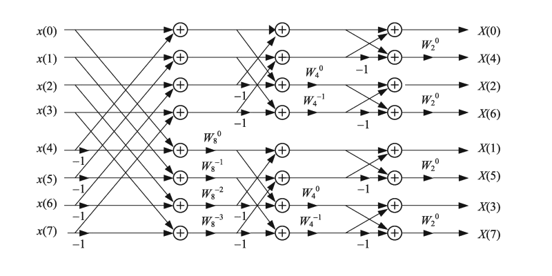
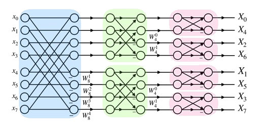
\(\begin{bmatrix}X(0)\\X(1)\\X(2)\\X(3)\\X(4)\\X(5)\\X(6)\\X(7)\end{bmatrix}=\begin{bmatrix}\omega^{0\times0}&\omega^{0\times1}&\omega^{0\times2}&\omega^{0\times3}&\omega^{0\times4}&\omega^{0\times5}&\omega^{0\times6}&\omega^{0\times7}\\\omega^{1\times0}&\omega^{1\times1}&\omega^{1\times2}&\omega^{1\times3}&\omega^{1\times4}&\omega^{1\times5}&\omega^{1\times6}&\omega^{1\times7}\\\omega^{2\times0}&\omega^{2\times1}&\omega^{2\times2}&\omega^{2\times3}&\omega^{2\times4}&\omega^{2\times5}&\omega^{2\times6}&\omega^{2\times7}\\\omega^{3\times0}&\omega^{3\times1}&\omega^{3\times2}&\omega^{3\times3}&\omega^{3\times4}&\omega^{3\times5}&\omega^{3\times6}&\omega^{3\times7}\\\omega^{4\times0}&\omega^{4\times1}&\omega^{4\times2}&\omega^{4\times3}&\omega^{4\times4}&\omega^{4\times5}&\omega^{4\times6}&\omega^{4\times7}\\\omega^{5\times0}&\omega^{5\times1}&\omega^{5\times2}&\omega^{5\times3}&\omega^{5\times4}&\omega^{5\times5}&\omega^{5\times6}&\omega^{5\times7}\\\omega^{6\times0}&\omega^{6\times1}&\omega^{6\times2}&\omega^{6\times3}&\omega^{6\times4}&\omega^{6\times5}&\omega^{6\times6}&\omega^{6\times7}\\\omega^{7\times0}&\omega^{7\times1}&\omega^{7\times2}&\omega^{7\times3}&\omega^{7\times4}&\omega^{7\times5}&\omega^{7\times6}&\omega^{7\times7}\end{bmatrix}\begin{bmatrix}x(0)\\x(1)\\x(2)\\x(3)\\x(4)\\x(5)\\x(6)\\x(7)\end{bmatrix}\)

\(=\begin{bmatrix}1&1&1&1&1&1&1&1\\1&\omega^1&\omega^2&\omega^3&\omega^4&\omega^5&\omega^6&\omega^7\\1&\omega^2&\omega^4&\omega^6&1&\omega^2&\omega^4&\omega^6\\1&\omega^3&\omega^6&\omega^1&\omega^4&\omega^7&\omega^2&\omega^5\\1&\omega^4&1&\omega^4&1&\omega^4&1&\omega^4\\1&\omega^5&\omega^2&\omega^7&\omega^4&\omega^1&\omega^6&\omega^3\\1&\omega^6&\omega^4&\omega^2&1&\omega^6&\omega^4&\omega^2\\1&\omega^7&\omega^6&\omega^5&\omega^4&\omega^3&\omega^2&\omega^1\end{bmatrix}\begin{bmatrix}x(0)\\x(1)\\x(2)\\x(3)\\x(4)\\x(5)\\x(6)\\x(7)\end{bmatrix}\), where \(\omega=e^{-j\frac{2\pi}8}\)

\(=\begin{bmatrix}1&1&1&1&1&1&1&1\\1&\omega^2&\omega^4&\omega^6&\omega^1&\omega^3&\omega^5&\omega^7\\1&\omega^4&1&\omega^4&\omega^2&\omega^6&\omega^2&\omega^6\\1&\omega^6&\omega^4&\omega^2&\omega^3&\omega^1&\omega^7&\omega^5\\1&1&1&1&\omega^4&\omega^4&\omega^4&\omega^4\\1&\omega^2&\omega^4&\omega^6&\omega^5&\omega^7&\omega^1&\omega^3\\1&\omega^4&1&\omega^4&\omega^6&\omega^2&\omega^6&\omega^2\\1&\omega^6&\omega^4&\omega^2&\omega^7&\omega^5&\omega^3&\omega^1\end{bmatrix}\begin{bmatrix}1&0&0&0&0&0&0&0\\0&0&1&0&0&0&0&0\\0&0&0&0&1&0&0&0\\0&0&0&0&0&0&1&0\\0&1&0&0&0&0&0&0\\0&0&0&1&0&0&0&0\\0&0&0&0&0&1&0&0\\0&0&0&0&0&0&0&1\end{bmatrix}\begin{bmatrix}x(0)\\x(1)\\x(2)\\x(3)\\x(4)\\x(5)\\x(6)\\x(7)\end{bmatrix}\)

\(=\begin{bmatrix}{\color[rgb]{0.0, 0.0, 1.0}1}&{\color[rgb]{0.0, 0.0, 1.0}1}&{\color[rgb]{0.0, 0.0, 1.0}1}&{\color[rgb]{0.0, 0.0, 1.0}1}&{\color[rgb]{1.0, 0.0, 0.0}1}&{\color[rgb]{1.0, 0.0, 0.0}1}&{\color[rgb]{1.0, 0.0, 0.0}1}&{\color[rgb]{1.0, 0.0, 0.0}1}\\{\color[rgb]{0.0, 0.0, 1.0}1}&\color[rgb]{0.0, 0.0, 1.0}\omega^2&\color[rgb]{0.0, 0.0, 1.0}\omega^4&\color[rgb]{0.0, 0.0, 1.0}\omega^6&\color[rgb]{1.0, 0.0, 0.0}\omega^1&\color[rgb]{1.0, 0.0, 0.0}\omega^3&\color[rgb]{1.0, 0.0, 0.0}\omega^5&\color[rgb]{1.0, 0.0, 0.0}\omega^7\\{\color[rgb]{0.0, 0.0, 1.0}1}&\color[rgb]{0.0, 0.0, 1.0}\omega^4&{\color[rgb]{0.0, 0.0, 1.0}1}&\color[rgb]{0.0, 0.0, 1.0}\omega^4&\color[rgb]{1.0, 0.0, 0.0}\omega^2&\color[rgb]{1.0, 0.0, 0.0}\omega^6&\color[rgb]{1.0, 0.0, 0.0}\omega^2&\color[rgb]{1.0, 0.0, 0.0}\omega^6\\{\color[rgb]{0.0, 0.0, 1.0}1}&\color[rgb]{0.0, 0.0, 1.0}\omega^6&\color[rgb]{0.0, 0.0, 1.0}\omega^4&\color[rgb]{0.0, 0.0, 1.0}\omega^2&\color[rgb]{1.0, 0.0, 0.0}\omega^3&\color[rgb]{1.0, 0.0, 0.0}\omega^1&\color[rgb]{1.0, 0.0, 0.0}\omega^7&\color[rgb]{1.0, 0.0, 0.0}\omega^5\\{\color[rgb]{0.68, 0.46, 0.12}1}&{\color[rgb]{0.68, 0.46, 0.12}1}&{\color[rgb]{0.68, 0.46, 0.12}1}&{\color[rgb]{0.68, 0.46, 0.12}1}&\color[rgb]{0.0, 0.0, 0.5}\omega^4&\color[rgb]{0.0, 0.0, 0.5}\omega^4&\color[rgb]{0.0, 0.0, 0.5}\omega^4&\color[rgb]{0.0, 0.0, 0.5}\omega^4\\{\color[rgb]{0.68, 0.46, 0.12}1}&\color[rgb]{0.68, 0.46, 0.12}\omega^2&\color[rgb]{0.68, 0.46, 0.12}\omega^4&\color[rgb]{0.68, 0.46, 0.12}\omega^6&\color[rgb]{0.0, 0.0, 0.5}\omega^5&\color[rgb]{0.0, 0.0, 0.5}\omega^7&\color[rgb]{0.0, 0.0, 0.5}\omega^1&\color[rgb]{0.0, 0.0, 0.5}\omega^3\\{\color[rgb]{0.68, 0.46, 0.12}1}&\color[rgb]{0.68, 0.46, 0.12}\omega^4&{\color[rgb]{0.68, 0.46, 0.12}1}&\color[rgb]{0.68, 0.46, 0.12}\omega^4&\color[rgb]{0.0, 0.0, 0.5}\omega^6&\color[rgb]{0.0, 0.0, 0.5}\omega^2&\color[rgb]{0.0, 0.0, 0.5}\omega^6&\color[rgb]{0.0, 0.0, 0.5}\omega^2\\{\color[rgb]{0.68, 0.46, 0.12}1}&\color[rgb]{0.68, 0.46, 0.12}\omega^6&\color[rgb]{0.68, 0.46, 0.12}\omega^4&\color[rgb]{0.68, 0.46, 0.12}\omega^2&\color[rgb]{0.0, 0.0, 0.5}\omega^7&\color[rgb]{0.0, 0.0, 0.5}\omega^5&\color[rgb]{0.0, 0.0, 0.5}\omega^3&\color[rgb]{0.0, 0.0, 0.5}\omega^1\end{bmatrix}P_8\begin{bmatrix}x(0)\\x(1)\\x(2)\\x(3)\\x(4)\\x(5)\\x(6)\\x(7)\end{bmatrix}\)

\(M_8=\begin{bmatrix}1&1&1&1&1&1&1&1\\1&\omega^2&\omega^4&\omega^6&\omega^1&\omega^3&\omega^5&\omega^7\\1&\omega^4&1&\omega^4&\omega^2&\omega^6&\omega^2&\omega^6\\1&\omega^6&\omega^4&\omega^2&\omega^3&\omega^1&\omega^7&\omega^5\\1&1&1&1&\omega^4&\omega^4&\omega^4&\omega^4\\1&\omega^2&\omega^4&\omega^6&\omega^5&\omega^7&\omega^1&\omega^3\\1&\omega^4&1&\omega^4&\omega^6&\omega^2&\omega^6&\omega^2\\1&\omega^6&\omega^4&\omega^2&\omega^7&\omega^5&\omega^3&\omega^1\end{bmatrix}P_8\)

\(=\begin{bmatrix}M_4&\begin{bmatrix}1&0&0&0\\0&\omega^1&0&0\\0&0&\omega^2&0\\0&0&0&\omega^3\end{bmatrix}M_4\\M_4&-\begin{bmatrix}1&0&0&0\\0&\omega^1&0&0\\0&0&\omega^2&0\\0&0&0&\omega^3\end{bmatrix}M_4\end{bmatrix}P_8=\begin{bmatrix}M_4&D_4M_4\\M_4&-D_4M_4\end{bmatrix}P_8\)

\(M_8=\begin{bmatrix}M_4&D_4M_4\\M_4&-D_4M_4\end{bmatrix}P_8=\begin{bmatrix}\begin{bmatrix}M_2&D_2M_2\\M_2&-D_2M_2\end{bmatrix}P_4&D_4\begin{bmatrix}M_2&D_2M_2\\M_2&-D_2M_2\end{bmatrix}P_4\\\begin{bmatrix}M_2&D_2M_2\\M_2&-D_2M_2\end{bmatrix}P_4&-D_4\begin{bmatrix}M_2&D_2M_2\\M_2&-D_2M_2\end{bmatrix}P_4\end{bmatrix}P_8\)

\(=\begin{bmatrix}\begin{bmatrix}M_2&D_2M_2\\M_2&-D_2M_2\end{bmatrix}&D_4\begin{bmatrix}M_2&D_2M_2\\M_2&-D_2M_2\end{bmatrix}\\\begin{bmatrix}M_2&D_2M_2\\M_2&-D_2M_2\end{bmatrix}&-D_4\begin{bmatrix}M_2&D_2M_2\\M_2&-D_2M_2\end{bmatrix}\end{bmatrix}\begin{bmatrix}P_4&0\\0&P_4\end{bmatrix}P_8\)

\(=\begin{bmatrix}I_4&D_4\\I_4&-D_4\end{bmatrix}\begin{bmatrix}I_2&D_2&0_{2,2}&0_{2,2}\\I_2&-D_2&0_{2,2}&0_{2,2}\\0_{2,2}&0_{2,2}&I_2&D_2\\0_{2,2}&0_{2,2}&I_2&-D_2\end{bmatrix}\begin{bmatrix}M_2&0_{2,2}&0_{2,2}&0_{2,2}\\0_{2,2}&M_2&0_{2,2}&0_{2,2}\\0_{2,2}&0_{2,2}&M_2&0_{2,2}\\0_{2,2}&0_{2,2}&0_{2,2}&M_2\end{bmatrix}\begin{bmatrix}P_4&0_{4,4}\\0_{4,4}&P_4\end{bmatrix}P_8\)

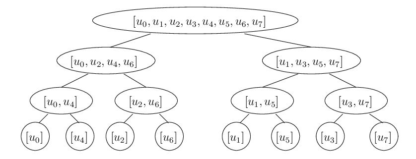
\(P_8\begin{bmatrix}x\lbrack0\rbrack\\x\lbrack1\rbrack\\x\lbrack2\rbrack\\x\lbrack3\rbrack\\x\lbrack4\rbrack\\x\lbrack5\rbrack\\x\lbrack6\rbrack\\x\lbrack7\rbrack\end{bmatrix}=\begin{bmatrix}1&0&0&0&0&0&0&0\\0&0&1&0&0&0&0&0\\0&0&0&0&1&0&0&0\\0&0&0&0&0&0&1&0\\0&1&0&0&0&0&0&0\\0&0&0&1&0&0&0&0\\0&0&0&0&0&1&0&0\\0&0&0&0&0&0&0&1\end{bmatrix}\begin{bmatrix}x\lbrack0\rbrack\\x\lbrack1\rbrack\\x\lbrack2\rbrack\\x\lbrack3\rbrack\\x\lbrack4\rbrack\\x\lbrack5\rbrack\\x\lbrack6\rbrack\\x\lbrack7\rbrack\end{bmatrix}=\begin{bmatrix}x\lbrack0\rbrack\\x\lbrack2\rbrack\\x\lbrack4\rbrack\\x\lbrack6\rbrack\\x\lbrack1\rbrack\\x\lbrack3\rbrack\\x\lbrack5\rbrack\\x\lbrack7\rbrack\end{bmatrix}\)

\(\begin{bmatrix}P_4&0_{4,4}\\0_{4,4}&P_4\end{bmatrix}\begin{bmatrix}x\lbrack0\rbrack\\x\lbrack2\rbrack\\x\lbrack4\rbrack\\x\lbrack6\rbrack\\x\lbrack1\rbrack\\x\lbrack3\rbrack\\x\lbrack5\rbrack\\x\lbrack7\rbrack\end{bmatrix}=\begin{bmatrix}1&0&0&0&0&0&0&0\\0&0&1&0&0&0&0&0\\0&1&0&0&0&0&0&0\\0&0&0&1&0&0&0&0\\0&0&0&0&1&0&0&0\\0&0&0&0&0&0&1&0\\0&0&0&0&0&1&0&0\\0&0&0&0&0&0&0&1\end{bmatrix}\begin{bmatrix}x\lbrack0\rbrack\\x\lbrack2\rbrack\\x\lbrack4\rbrack\\x\lbrack6\rbrack\\x\lbrack1\rbrack\\x\lbrack3\rbrack\\x\lbrack5\rbrack\\x\lbrack7\rbrack\end{bmatrix}=\begin{bmatrix}x\lbrack0\rbrack\\x\lbrack4\rbrack\\x\lbrack2\rbrack\\x\lbrack6\rbrack\\x\lbrack1\rbrack\\x\lbrack5\rbrack\\x\lbrack3\rbrack\\x\lbrack7\rbrack\end{bmatrix}\)

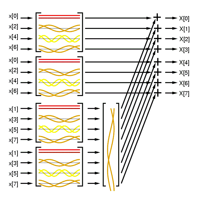
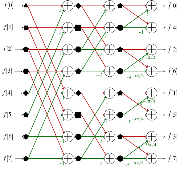
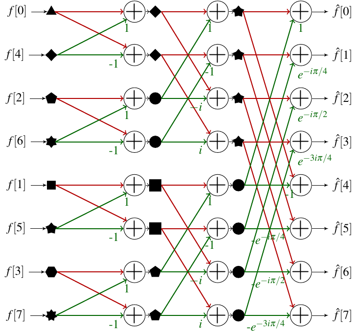
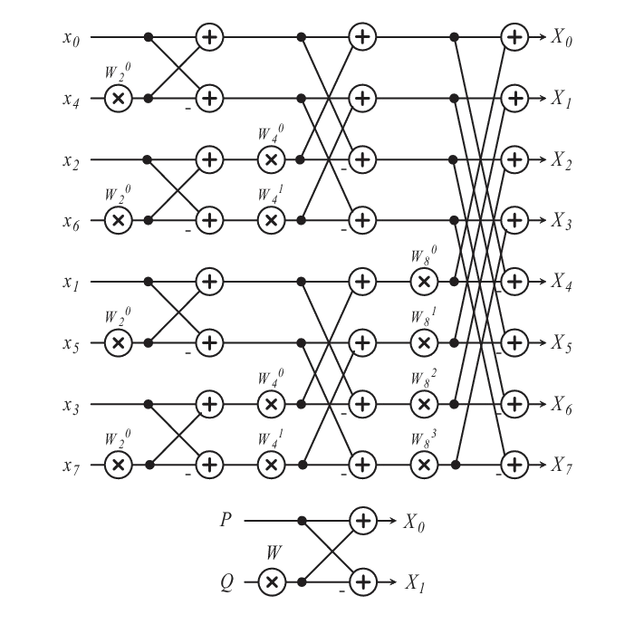
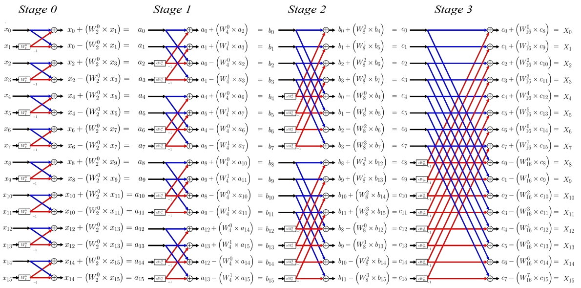
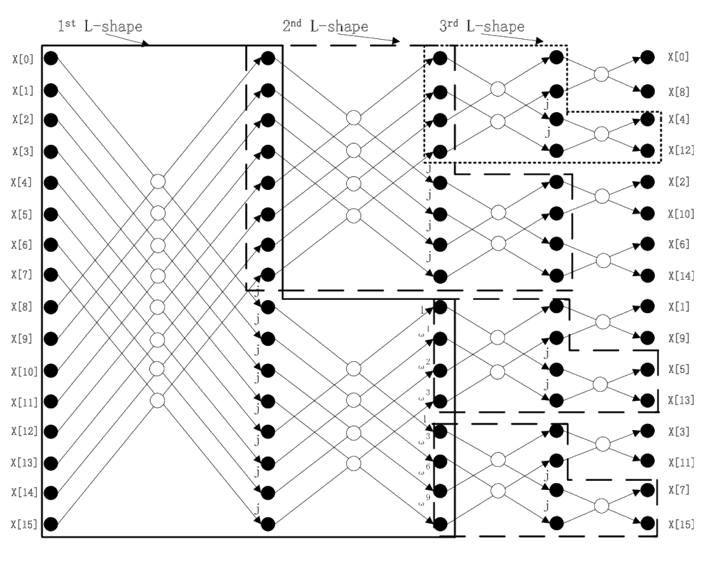
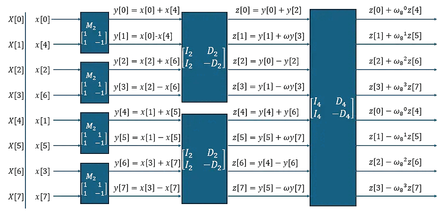
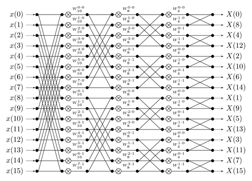
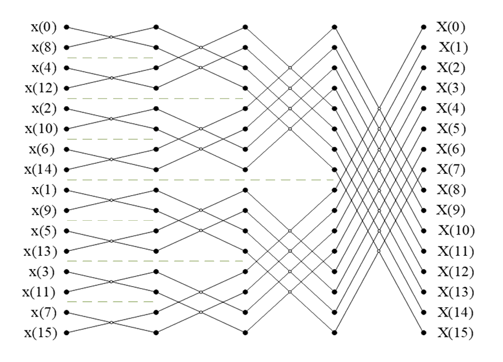
\(\begin{bmatrix}X\lbrack0\rbrack\\X\lbrack1\rbrack\\X\lbrack2\rbrack\\X\lbrack3\rbrack\\X\lbrack4\rbrack\\X\lbrack5\rbrack\\X\lbrack6\rbrack\\X\lbrack7\rbrack\end{bmatrix}=\begin{bmatrix}I_4&D_4\\I_4&-D_4\end{bmatrix}\begin{bmatrix}I_2&D_2&0_{2,2}&0_{2,2}\\I_2&-D_2&0_{2,2}&0_{2,2}\\0_{2,2}&0_{2,2}&I_2&D_2\\0_{2,2}&0_{2,2}&I_2&-D_2\end{bmatrix}\begin{bmatrix}M_2&0_{2,2}&0_{2,2}&0_{2,2}\\0_{2,2}&M_2&0_{2,2}&0_{2,2}\\0_{2,2}&0_{2,2}&M_2&0_{2,2}\\0_{2,2}&0_{2,2}&0_{2,2}&M_2\end{bmatrix}\begin{bmatrix}x\lbrack0\rbrack\\x\lbrack1\rbrack\\x\lbrack2\rbrack\\x\lbrack3\rbrack\\x\lbrack4\rbrack\\x\lbrack5\rbrack\\x\lbrack6\rbrack\\x\lbrack7\rbrack\end{bmatrix}\)

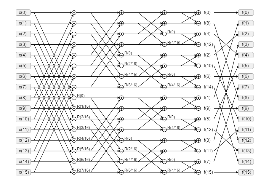
FFT complexity

\(X_n=\sum_{k=0}^{\frac N2-1}x_{2n}⋅e^{\frac{-i⋅2\pi⋅k⋅n}{N/2}}+e^{\frac{-i⋅2\pi⋅n}N}\sum_{k=0}^{\frac N2-1}x_{2n+1}⋅e^{\frac{-i⋅2\pi⋅k⋅n}{N/2}}\)

\({\frac n{n_1}}O(n_1\log\;n_1)+\cdots+{\frac n{n_d}}O(n_d\log\;n_d)\)

\(=O{(n{\lbrack\log\;n_1+\cdots+\log\;n_d\rbrack})}=O(n\log\;n)\)

taking FFTs -- \(O(N \log N)\)
multiplying FFTs -- \(O(N)\)
inverse FFTs -- \(O(N \log N)\).
the total complexity is \(O(N \log N)\).

Time weighting windows

FFT Analyzers use time-weighting window functions to reduce spectral leakage. Such leakage phenomena cause amplitude errors in the frequency spectrum.

Spectral leakage

Spectral leakage is when the energy of frequency components in a signal is spread out to a broad range of spectral lines instead of being represented by single spectral lines.

Spectral leakage is the spreading of a signal's energy across neighboring frequencies in a Fourier transform analysis. This phenomenon occurs when a signal's frequency is not an integer multiple of the sampling rate, causing it to appear in more frequency bins than just its true frequency. To mitigate spectral leakage, you can apply window functions to the signal or record a longer segment of the signal to increase frequency resolution.

Windowing a sinusoid causes spectral leakage, even if the sinusoid has an integer number of cycles within a rectangular window. The leakage is evident in the 2nd row, blue trace. It is the same amount as the red trace, which represents a slightly higher frequency that does not have an integer number of cycles. When the sinusoid is sampled and windowed, its discrete-time Fourier transform also exhibits the same leakage pattern (rows 3 and 4). But when the DTFT is only sparsely sampled, at a certain interval, it is possible (depending on your point of view) to: (1) avoid the leakage, or (2) create the illusion of no leakage. For the case of the blue sinusoid DTFT (3rd row of plots, right-hand side), those samples are the outputs of the discrete Fourier transform (DFT). The red sinusoid DTFT (4th row) has the same interval of zero-crossings, but the DFT samples fall in-between them, and the leakage is revealed.

Two different ways to generate an 8-point Gaussian window sequence (σ = 0.4) for spectral analysis applications. MATLAB calls them "symmetric" and "periodic". The latter is also historically called DFT-even.

Spectral leakage characteristics of the functions in previous figure.

Concept of window functions

Time weighting techniques add a “window” with individual weighting coefficients to each time sample in an FFT time block. This primarily reduces those samples that cause spectral leakage. In effect, samples at the time block ends are reduced to zero (or heavily reduced), so that the discontinuities in the periodized time signal are removed.

Effective noise bandwidth (NBW)

The NBW (also referred to as the “Effective Noise Bandwidth”) is defined as the width of an ideal filter that transmits the same power from a white noise source as the given/used filter

The figure of a used practical filter and an ideal filter. The ideal filter transmits all frequency components contained within its NBW and removes all other components.

Ripple (max. amplitude error)

Ripple, also referred to as Flatness or Scalloping Loss indicates the maximum amplitude error within \(\pm\frac{\Delta f}2\) around a spectral line, and thereby determines the accuracy of the amplitude of the signal. This maximum amplitude error is also referred to as the maximum picket fence effect error.

Window functions do not completely remove spectral leakage, and sidelobes will still exist, but they are more attenuated. The selectivity parameters that describe such sidelobe characteristics are illustrated in the picture below:

Window types

The choice of which window function to use depends upon the frequency content of the signal. Some window functions have a relatively small NBW (Noise BandWidth) which provides good Frequency Resolution \(f_{NBW}\), like the Hanning window.
Good frequency resolution is desired for signals containing closely spaced frequency components of interest with similar amplitude levels.
Other window functions have greater \(NBW\) like the Flattop window, however Flat top performs better in the determination of exact amplitude levels due to its low ripple value.
If two closely spaced tones with very different amplitude levels need to be separable, then window functions with good selectivity should be used. For example, if you have a narrow 60 dB bandwidth and a small value for the highest sidelobe, it is more likely that the weak tonal component will be detectable from the energy spreading of the strong tonal component.
Illustrations below show simulations of some common window functions and their differences with respect to the NBW, ripple, and selectivity.

Simulations of commonly used window functions, indicating their different characteristics which are used to select which window to use for a certain analysis scenario.

Simulations of commonly used window functions, showing their sidelobe fall-off rate.

From the window function simulations illustrated above, the characteristic parameters for window functions can be determined. See the table below:

Extract amplitude of frequency components (amplitude spectrum)

The FFT function computes the complex DFT and the hence the results in a sequence of complex numbers of form \(X_{re} + j X_{im}\). The amplitude spectrum is obtained

\[|X[k]| = \sqrt{X_{re}^2 + X_{im}^2 } \]

Extract phase of frequency components (phase spectrum)

Extracting the correct phase spectrum is a tricky business. I will show you why it is so. The phase of the spectral components are computed as

\[\angle X[k] = tan^{-1} \left( \frac{X_{im}}{X_{re}} \right)\]

yahoo

ABCD