the Operations in Geometric Algebra
Products:
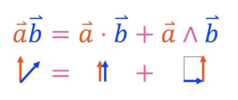
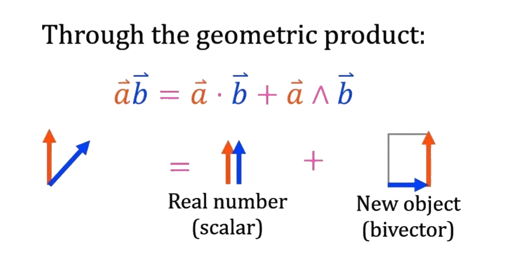
- Geometric Product \( (AB = A \cdot B + A \wedge B) \)
- Outer Product \( (\wedge) \)
- Regressive Product \( (\vee) \)
- Inner Product \( (\cdot) \)
Involutions:
- Reverse \( (A^\dagger \text{ or } \tilde{A}) \)
- Grade involution \( (\hat{A}) \)
Other operations:
- Dual \( (A^*) \)
- Grade Projection \( (\langle A \rangle_k) \)
- Magnitude \( (|A|) \)
- Vanilla Geometric Algebra \( (\text{VGA}) \)
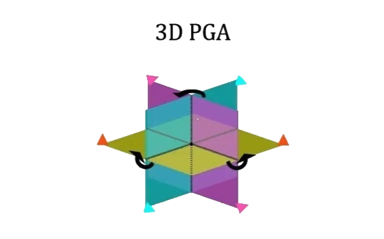
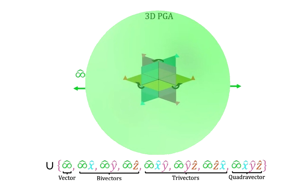
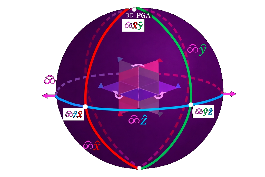
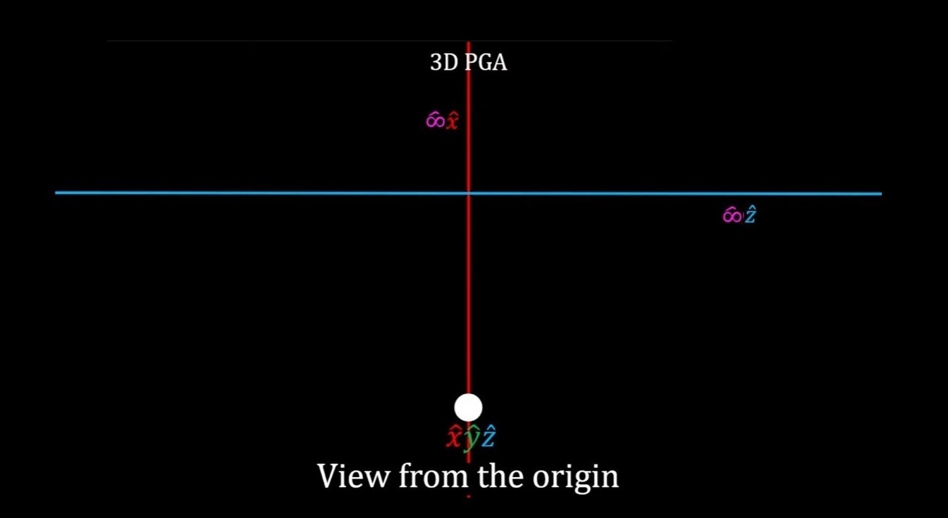
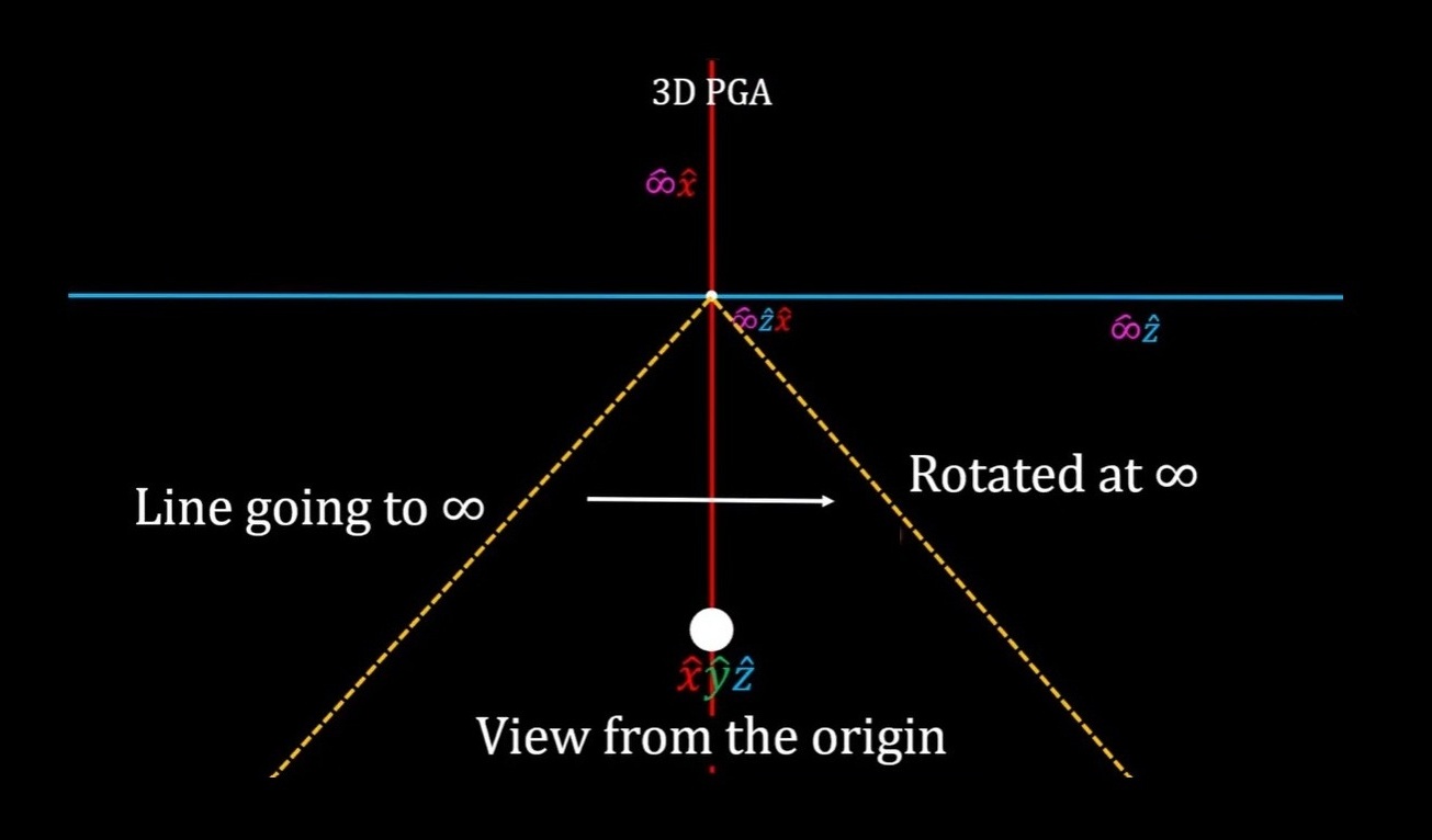
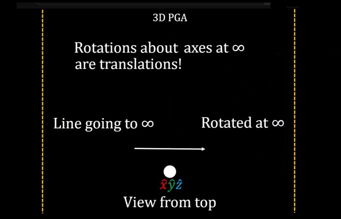
- Projective Geometric Algebra \( (\text{PGA}) \)
- Conformal Geometric Algebra \( (\text{CGA}) \)
- Spacetime Algebra \( (\text{STA}) \)
- \( \vdots \)
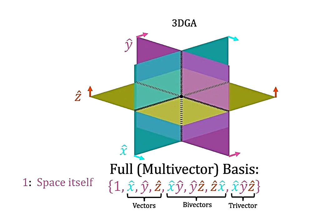
Multivectors
- Vectors
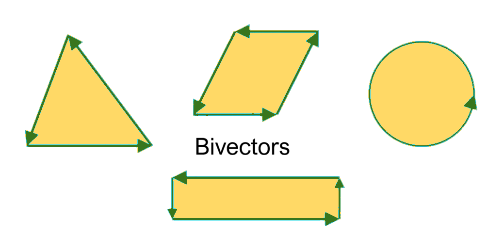
- Bivectors
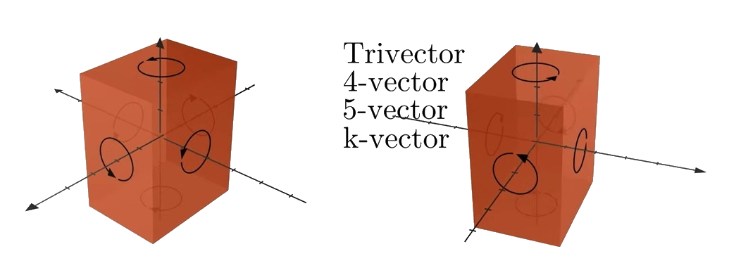
- Trivectors
- \( \vdots \)

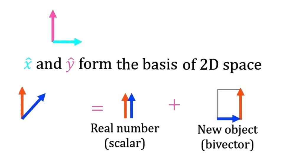
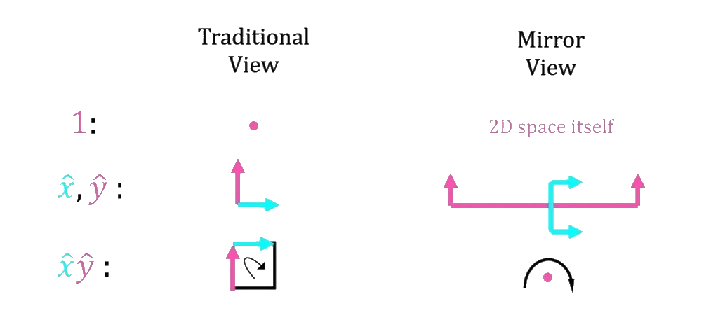
Vanilla Geometric Algebra (VGA), often referred to as vector-space geometric algebra, is the most fundamental foundation of geometric algebra.
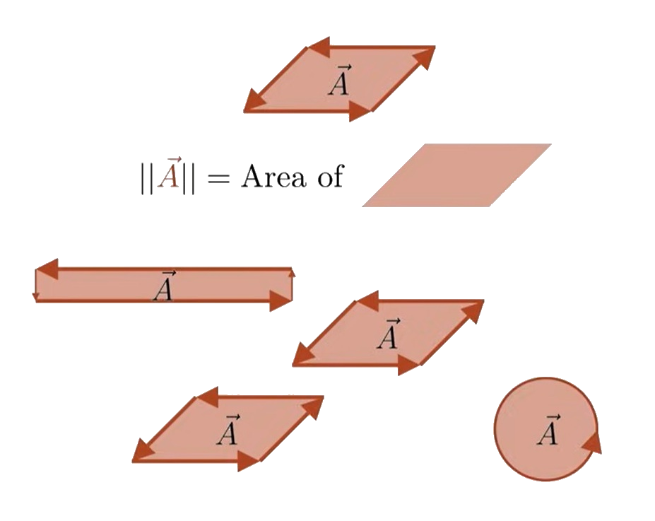
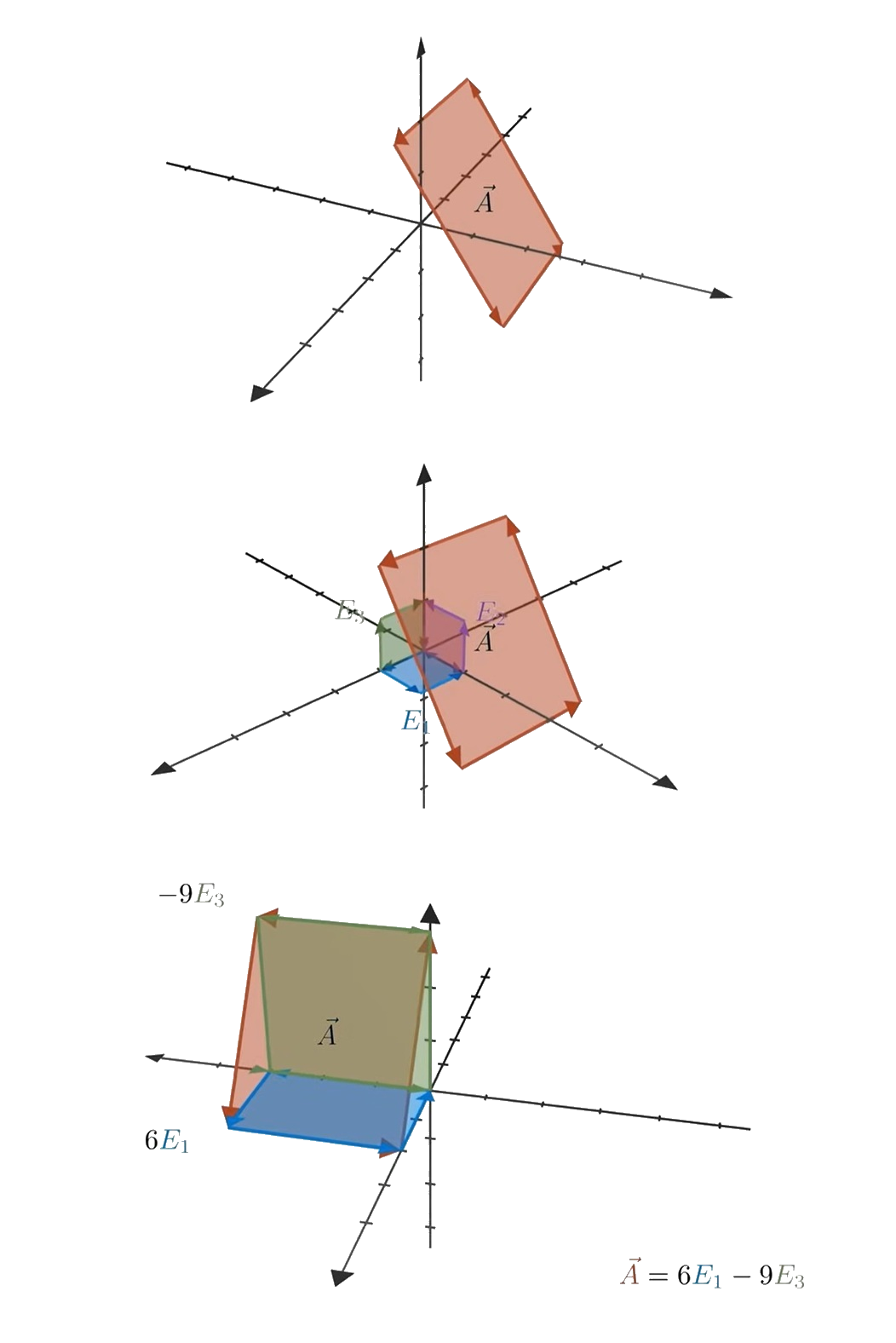
Bivector
\( \text{Plane} \) \(\text{(Two-Dimensional Subspace)}\)
\( \text{Orientation} \)
\( \text{Magnitude} \)
| \( \text{Vector:} \) |
\( \text{One-Dimensional Subspace} \) |
| \( \text{Bivector:} \) |
\( \text{Two-Dimensional Subspace} \) |
| \( \text{Trivector:} \) |
\( \text{Three-Dimensional Subspace} \) |
| \( \vdots \) |
\( \vdots \) |
| \( k\text{-vector:} \) |
\( k\text{-Dimensional Subspace} \) |
\( \text{Multivector:} \quad \text{Scalar} + \text{Vector} + \cdots + k\text{-vector} \)
Grade Projection Operator
\( \langle A \rangle_k = \text{The } k\text{-vector part of } A \)
\( a + b e_1 + c e_2 + d e_1 e_2 \)
\( \langle a + b e_1 + c e_2 + d e_1 e_2 \rangle = a \)
\( \langle a + b e_1 + c e_2 + d e_1 e_2 \rangle_1 = b e_1 + c e_2 \)
\( \langle a + b e_1 + c e_2 + d e_1 e_2 \rangle_2 = d e_1 e_2 \)
\( \langle A \rangle_k = \text{The } k\text{-vector part of } A \)
\( \text{When } A \text{ only has a } k\text{-vector component,} \) \( A \text{ has a grade of } k. \)
Scalars are grade zero objects
Vectors are grade one objects
Bivectors are grade two objects
\( \vdots \)
Geometric Product
Geometric
Algebraic
Transformations
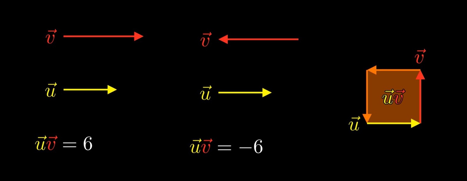
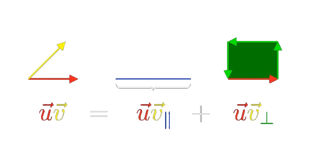
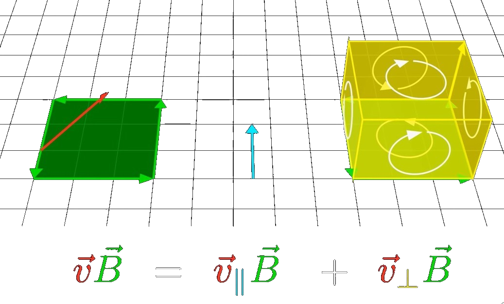
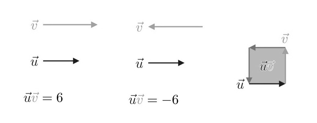
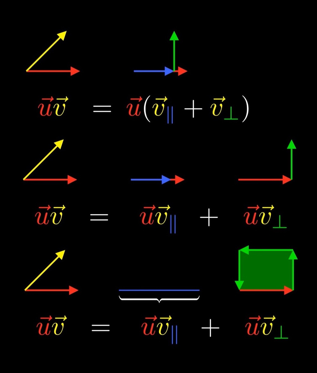
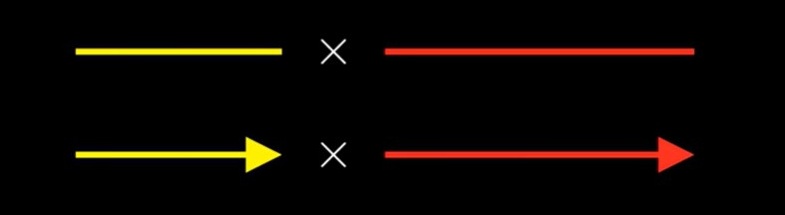
The geometric product
contracts parallel directions
and joins perpendicular directions.
\( e_1, e_2, e_3, \cdots, e_n \)
\( e_i e_j = -e_j e_i \)
\( (i \neq j) \)
\( e_i^2 = 1? \)
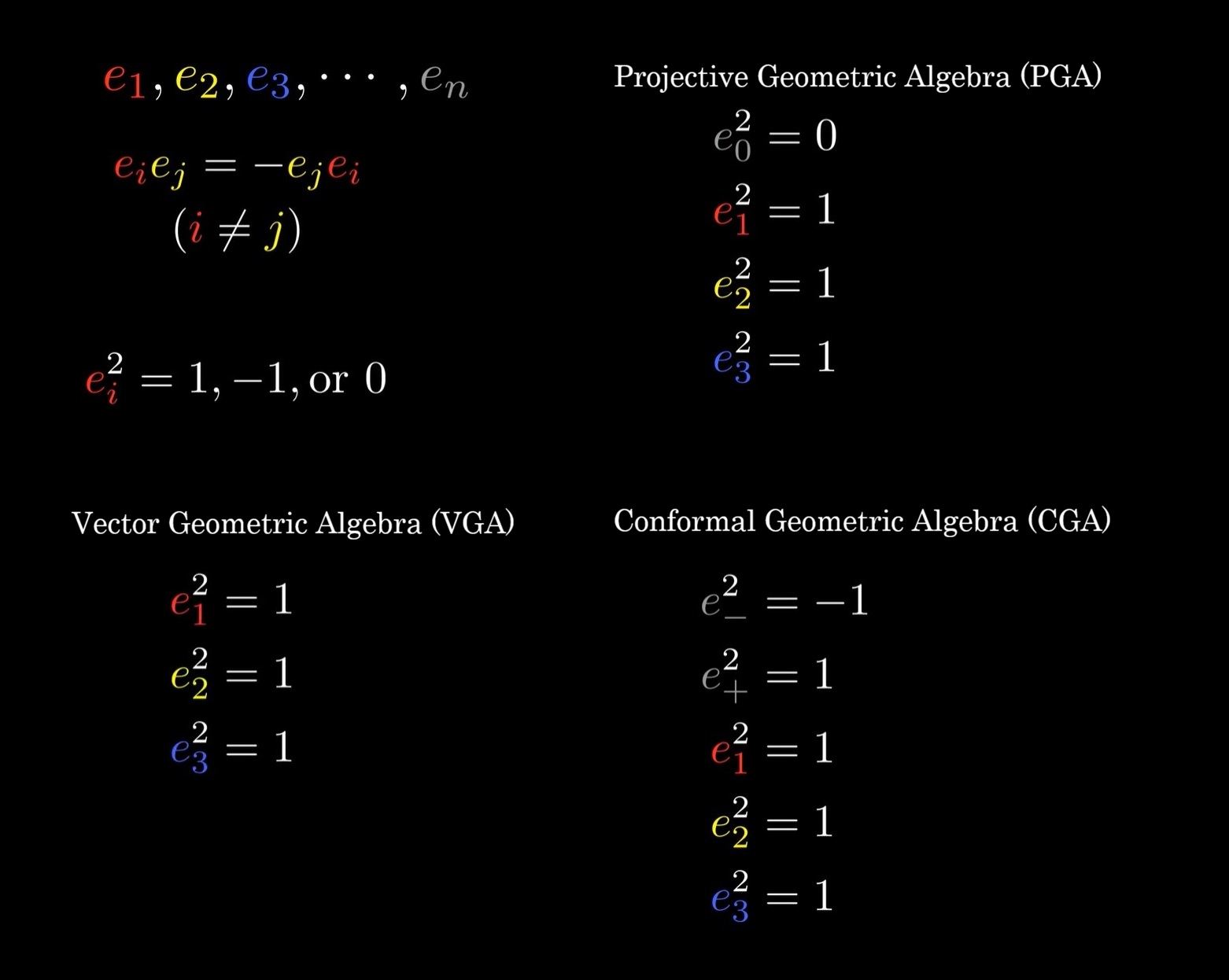
\( \mathbb{G}(p, q, r) \text{ or } \text{Cl}(p, q, r) \)
\( p \) basis vectors square to 1
\( q \) basis vectors square to -1
\( r \) basis vectors square to 0
\( \mathbb{G}(1,1,1) \quad e_1^2 = 1 \quad e_2^2 = -1 \quad e_0^2 = 0 \)
[Ex] \( (e_1 - e_0 e_2)(2 + e_1 e_2 - e_0 e_1) \)
\( = 2e_1 + e_1 e_1 e_2 - e_1 e_0 e_1 - 2e_0 e_2 - e_0 e_2 e_1 e_2 + e_0 e_2 e_0 e_1 \)
\( = 2e_1 + e_1 e_1 e_2 + e_0 e_1 e_1 - 2e_0 e_2 + e_0 e_1 e_2 e_2 - e_0 e_0 e_2 e_1 \)
\( = 2e_1 + e_2 + e_0 - 2e_0 e_2 + e_0 e_1 e_2 e_2 - e_0 e_0 e_2 e_1 \)
\( = 2e_1 + e_2 + e_0 - 2e_0 e_2 - e_0 e_1 - e_0 e_0 e_2 e_1 \)
\( = 2e_1 + e_2 + e_0 - 2e_0 e_2 - e_0 e_1 \)
\( = 2e_1 + e_2 + e_0 - 2e_{02} - e_0 e_1 \)
\( = 2e_1 + e_2 + e_0 - 2e_{02} - e_{01} \)
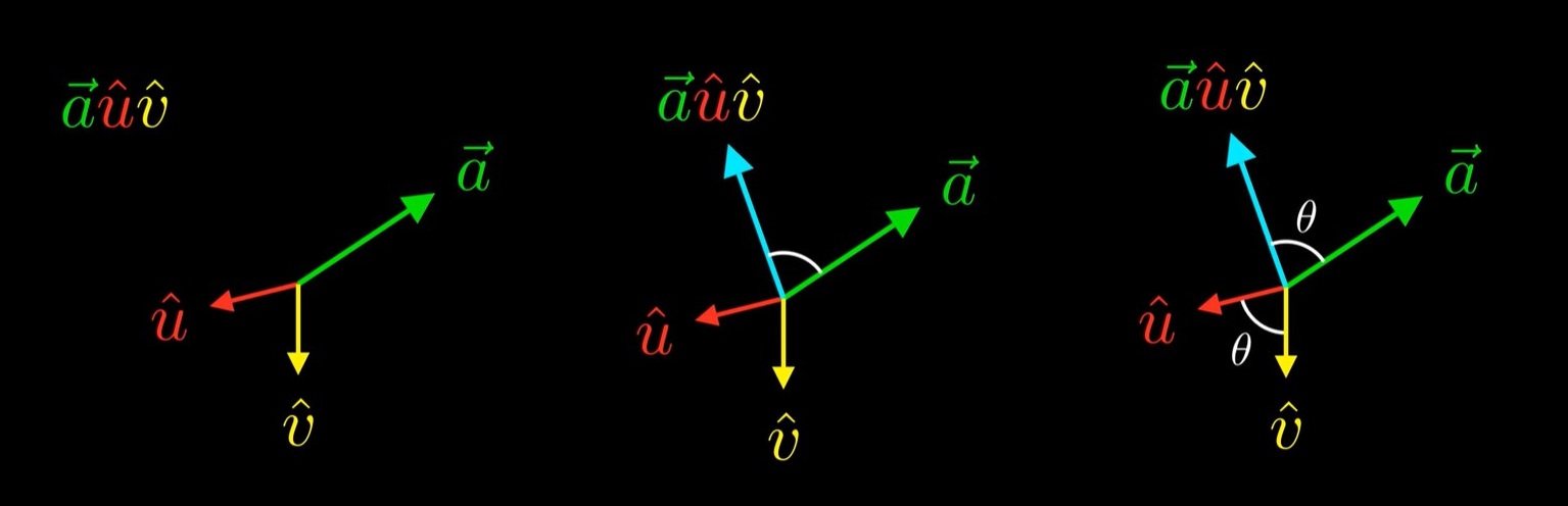
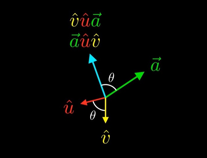
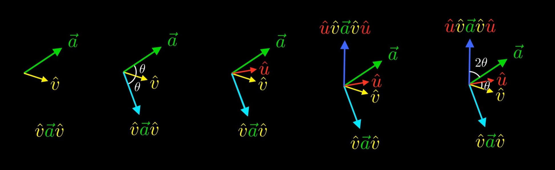
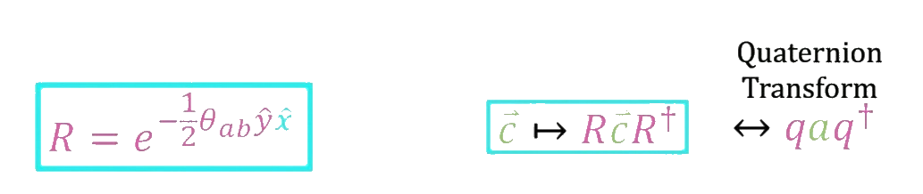
\( \hat{v}\vec{a}\hat{v} \)
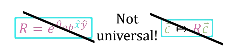
\( \text{in higher Dimensions the simple rotation formula doesn't hold but the reflection formula does hold} \).
\( \dots \hat{w}\hat{u}\hat{v}\vec{a}\hat{v}\hat{u}\hat{w} \dots \)
You can get any orthogonal transformation this way.
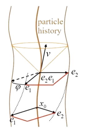
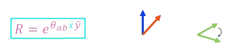
\( \vec{a}\hat{u}\hat{v} \quad \text{2D Rotation} \)
\( \hat{u}\vec{a}\hat{u} \quad \text{Reflection} \)
\( \dots \hat{w}\hat{u}\hat{v}\vec{a}\hat{v}\hat{u}\hat{w} \dots \quad \text{Orthogonal Transformation} \)
Reverse
\( \vec{u}\vec{v}\vec{w} \xrightarrow{\text{Reverse}} \vec{w}\vec{v}\vec{u} \)
\( (\vec{u}\vec{v}\vec{w})^\dagger = \vec{w}\vec{v}\vec{u} \)
\( (1 + 2e_1 + e_{12} + 3e_{123} + e_{1234})^\dagger \)
\(= 1^\dagger + 2e_1^\dagger + e_{12}^\dagger + 3e_{123}^\dagger + e_{1234}^\dagger \)
\(= 1 + 2e_1 + e_{21} + 3e_{321} + e_{4321} \)
\(= 1 + 2e_1 - e_{12} + 3e_{321} + e_{4321} \)
\(= 1 + 2e_1 - e_{12} - 3e_{231} + e_{4321} \)
\(= 1 + 2e_1 - e_{12} + 3e_{213} + e_{4321} \)
\(= 1 + 2e_1 - e_{12} - 3e_{123} + e_{4321} \)
\(= 1 + 2e_1 - e_{12} - 3e_{123} - e_{3421} \)
\(= 1 + 2e_1 - e_{12} - 3e_{123} + e_{3241} \)
\(= 1 + 2e_1 - e_{12} - 3e_{123} - e_{3214} \)
\(= 1 + 2e_1 - e_{12} - 3e_{123} + e_{2314} \)
\(= 1 + 2e_1 - e_{12} - 3e_{123} - e_{2134} \)
\(= 1 + 2e_1 - e_{12} - 3e_{123} + e_{1234} \)
\( 1 + 2e_1 + e_{21} + 3e_{321} + e_{4321} \)
\(= 1 + 2e_1 - e_{12} - 3e_{123} + e_{1234} \)
Reverse
\( \text{0-Vector} \quad + \)
\( \text{1-Vector} \quad + \)
\( \text{2-Vector} \quad - \)
\( \text{3-Vector} \quad - \)
\( \text{4-Vector} \quad + \)
\( \text{5-Vector} \quad + \)
\( \text{6-Vector} \quad - \)
\( \text{7-Vector} \quad - \)
Grade Involution
\( \text{0-Vector} \quad + \)
\( \text{1-Vector} \quad - \)
\( \text{2-Vector} \quad + \)
\( \text{3-Vector} \quad - \)
\( \text{4-Vector} \quad + \)
\( \text{5-Vector} \quad - \)
\( \text{6-Vector} \quad + \)
\( \text{7-Vector} \quad - \)
Grade Involution
\( A^* \qquad \hat{A} \)
Confused of \( \text{Dual of } A\text{: } A^* \)
\( \text{Unit vector: } \hat{a} \)
\( (\vec{u}\vec{v}\vec{w})^\wedge \)
\( \text{Dual of } A\text{: } \star A \)
Grade Involution
\( A^* \)
\( (A + B)^* = A^* + B^* \)
\( (\alpha A)^* = \alpha A^* \)
\( (AB)^* = A^* B^* \)
\( (1 + 2e_1 + e_{12} + 3e_{123} + e_{1234})^* \)
\( = 1 - 2e_1 + e_{12} - 3e_{123} + e_{1234} \)
Magnitude
\( |\alpha| = \sqrt{\alpha^2} \qquad |\vec{v}| = \sqrt{\vec{v}^2} \)
\( |A| = \sqrt{A^2} \)
\( |A|^2 = A^2 \)
\( |e_{12}|^2 = 1 \qquad e_{12}^2 = -1 \)
\( |A|^2 = A^\dagger A \)
\( |e_{12}|^2 = 1 \)
\( |e_{12}|^2 = (e_1 e_2)^\dagger e_1 e_2 \)
\( |e_{12}|^2 = e_2 e_1 e_1 e_2 \)
\( |e_{12}|^2 = e_2 e_2 \)
\( |e_{12}|^2 = 1 \)
\( |A|^2 = A^\dagger A \)
\( |1 + e_1|^2 = 2 + 2e_1 \)
\( |A|^2 = \langle A^\dagger A \rangle \)
\( |1 + e_1|^2 = 2 \)
\( |A|^2 = \langle A^\dagger A \rangle \)
\( |a + be_1 + ce_2 + de_{12}|^2 = a^2 + b^2 + c^2 + d^2 \)
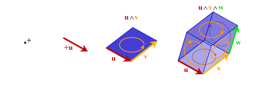
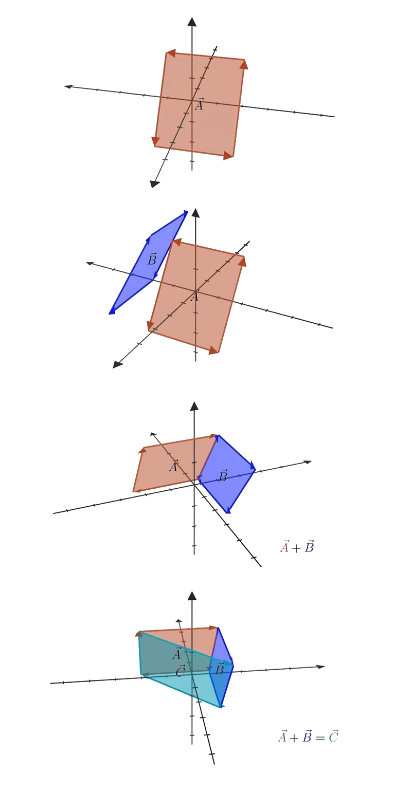
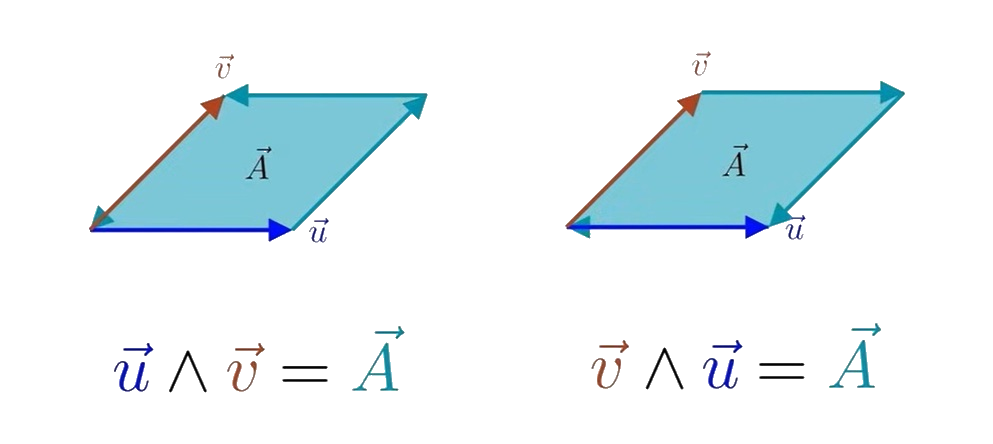
Outer Product
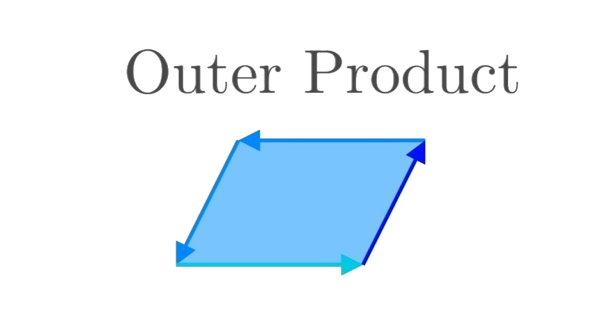
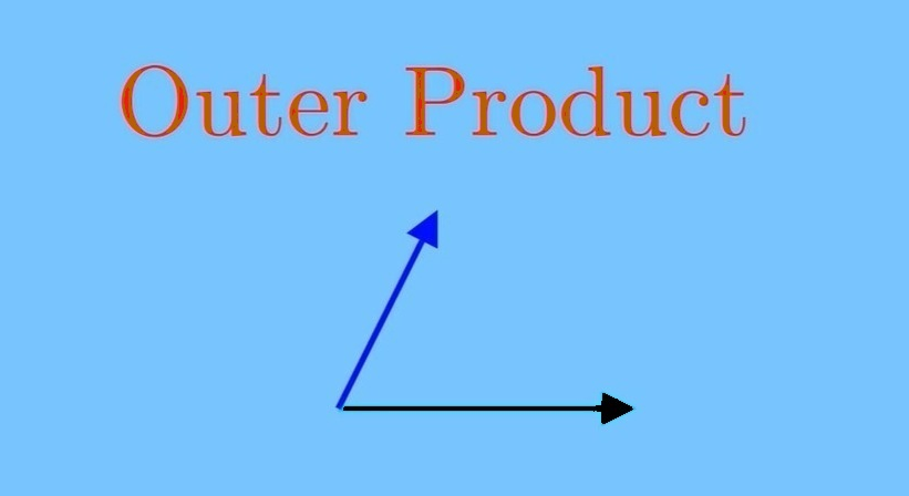
\( \vec{u} \wedge \vec{v} \) represents the span of \( \vec{u} \) and \( \vec{v} \)
\( \vec{v} \wedge \vec{v} = 0 \)
If the span of \( \vec{v}_1, \cdots, \) and \( \vec{v}_n \) is \( n \)-dimensional, \( \vec{v}_1 \wedge \cdots \wedge \vec{v}_n \) represents the span of \( \vec{v}_1, \cdots, \) and \( \vec{v}_n \)
If \( \vec{v}_1, \cdots, \) and \( \vec{v}_n \) are linearly independent, \( \vec{v}_1 \wedge \cdots \wedge \vec{v}_n \) represents the span of \( \vec{v}_1, \cdots, \) and \( \vec{v}_n \)
Outer Product
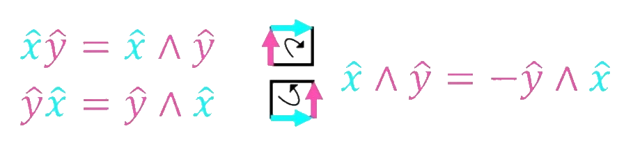
\( e_i \wedge e_j = -e_j \wedge e_i \)
\( e_i e_j = -e_j e_i \)
\( e_i \wedge e_i = 0 \)
\( e_i e_i = -1, 0, \text{ or } 1 \)
\( (e_{01} + e_{56}) \wedge (e_{1234} + e_{3456}) \)
\( e_{01} \wedge e_{1234} + e_{01} \wedge e_{3456} + e_{56} \wedge e_{1234} + e_{56} \wedge e_{3456} \)
\( = 0 + e_{01} \wedge e_{3456} + e_{56} \wedge e_{1234} + e_{56} \wedge e_{3456} \)
\( = e_{01} \wedge e_{3456} + e_{56} \wedge e_{1234} + e_{56} \wedge e_{3456} \)
\( = e_{01} \wedge e_{3456} + e_{56} \wedge e_{1234} + 0 \)
\( = e_{01} \wedge e_{3456} + e_{56} \wedge e_{1234} \)
\( = e_{013456} + e_{561234} \)
\( = e_{013456} + e_{123456} \)
\( (e_{01} + e_{56}) \wedge (e_{1234} + e_{3456}) \)
\( e_{013456} + e_{123456} \)
\( \text{j-vector} \wedge \text{k-vector} = (j + k)\text{-vector} \)
Outer Product
\( (e_{01} + e_{56}) \wedge (e_{1234} + e_{3456}) \)
\( e_{013456} + e_{123456} \)
\( (e_{01} + e_{56})(e_{1234} + e_{3456}) \)
\( -e_{34} + e_{0234} + e_{013456} + e_{123456} \)
\( (e_{01} + e_{56})(e_{1234} + e_{3456}) = e_{01}e_{1234} + e_{01}e_{3456} + e_{56}e_{1234} + e_{56}e_{3456} \)
\( = (e_0 e_1)(e_1 e_2 e_3 e_4) + (e_0 e_1)(e_3 e_4 e_5 e_6) + (e_5 e_6)(e_1 e_2 e_3 e_4) + (e_5 e_6)(e_3 e_4 e_5 e_6) \)
\( = e_0 (e_1 e_1) e_2 e_3 e_4 + e_0 e_1 e_3 e_4 e_5 e_6 + (-1)^8(e_1 e_2 e_3 e_4 e_5 e_6) + e_5 e_6 e_3 e_4 e_5 e_6 \)
\( = e_{0234} + e_{013456} + e_{123456} + (-1)(e_5 e_3 e_6 e_4 e_5 e_6) \)
\( = e_{0234} + e_{013456} + e_{123456} + (+1)(e_3 e_5 e_6 e_4 e_5 e_6) \)
\( = e_{0234} + e_{013456} + e_{123456} + (-1)(e_3 e_5 e_4 e_6 e_5 e_6) \)
\( = e_{0234} + e_{013456} + e_{123456} + (+1)(e_3 e_4 e_5 e_6 e_5 e_6) \)
\( = e_{0234} + e_{013456} + e_{123456} + (-1)(e_3 e_4 e_5 e_5 e_6 e_6) \)
\( = e_{0234} + e_{013456} + e_{123456} - e_3 e_4 (1) (1) \)
\( = e_{0234} + e_{013456} + e_{123456} - e_{34} \)
\( = -e_{34} + e_{0234} + e_{013456} + e_{123456} \)

Regressive Product
The regressive product (usually referred to as the "meet") is the dual of the exterior product (or "join" in this context)
Outer Product
\( A_j \wedge B_k = \langle A_j B_k \rangle_{j+k} \)
Outer Product
Span
Outer Product
\( A \wedge B \)
Smallest subspace containing the inputs
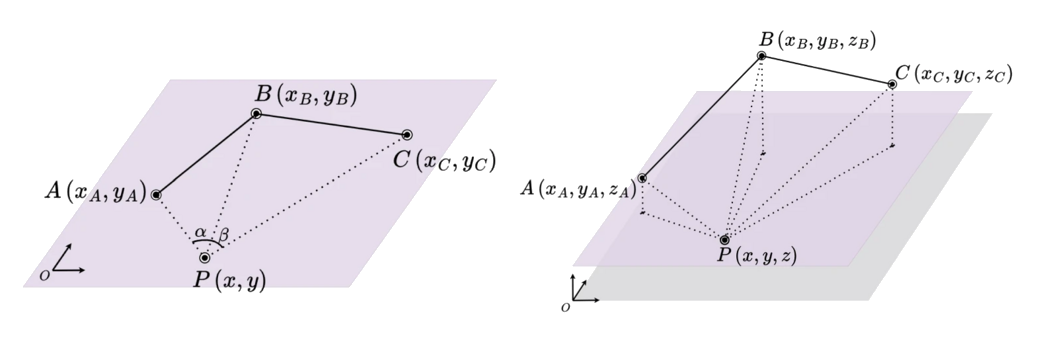
Regressive Product
\( A \vee B \)
Largest subspace contained in the inputs
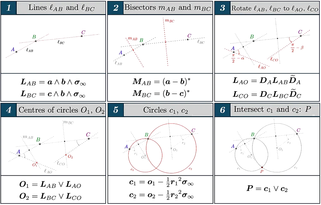
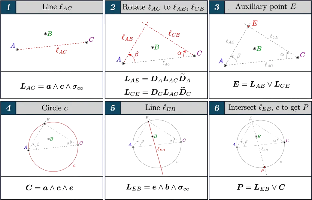
In Geometric algebra, the regressive product (often denoted as \(\vee\)) is the dual of the exterior/wedge product (\(\wedge\)). While the exterior product represents the "join" (spanning) of two subspaces, the regressive product represents their geometric intersection (the "meet").
Core Concepts
-
The Join and Meet: If you take the exterior product of two points \(P\) and \(Q\) to form a line, you get the join: \(P \wedge Q = \text{line}\). If you take the regressive product of two lines, you get their point of intersection: \(\text{line}_1 \vee \text{line}_2 = \text{point}\).
-
Duality: The regressive product can be explicitly computed using the exterior product and the algebraic complement (or duality) operator denoted as \(\sim\). For multivectors \(A\) and \(B\), the regressive product is defined as:
\(A \vee B = \sim (\sim A \wedge \sim B)\)
The dual specification of elements permits, for blades \(A\) and \(B\), the intersection (or meet) where the duality is to be taken relative to the smallest grade blade containing both \(A\) and \(B\) (the join).
\( C \vee D := ((CI^{-1}) \wedge (DI^{-1}))I \)
with \(I\) the unit pseudoscalar of the algebra. The regressive product, like the exterior product, is associative.
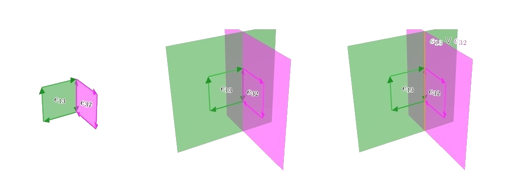
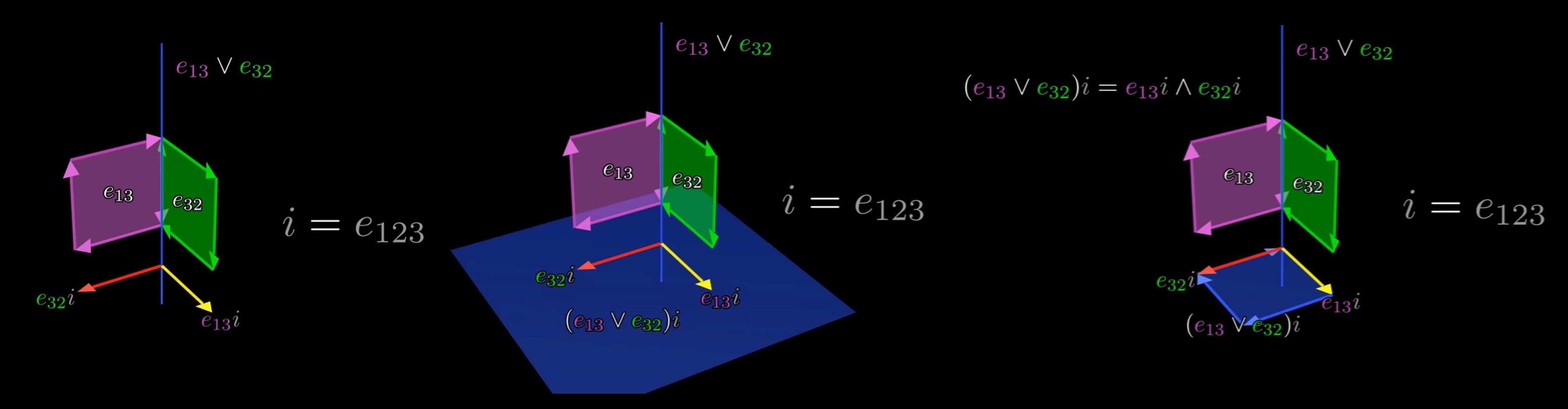
\( (A \vee B)i = Ai \wedge Bi \)
\( A \vee B = (Ai \wedge Bi)i^{-1} \)
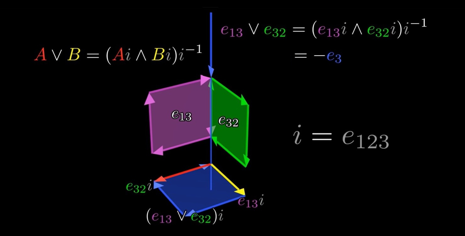
\( e_{13} \vee e_{32} = (e_{13}i \wedge e_{32}i)i^{-1} \)
\( e_{13} \vee e_{32} = (e_2 \wedge e_1)i^{-1} \)
\( e_{13} \vee e_{32} = e_{21}i^{-1} \)
\( e_{13} \vee e_{32} = -e_3 \)
\( A \vee B = (Ai \wedge Bi)i^{-1} \)
In three dimensions: \( e_{13} \vee e_{32} = -e_3 \)
In four dimensions: \( e_{13} \vee e_{32} = (e_{13}i \wedge e_{32}i)i^{-1} \)
In four dimensions: \( e_{13} \vee e_{32} = (e_{24} \wedge e_{14})i^{-1} \)
\( = (0)i^{-1} \)
\( = 0 \)
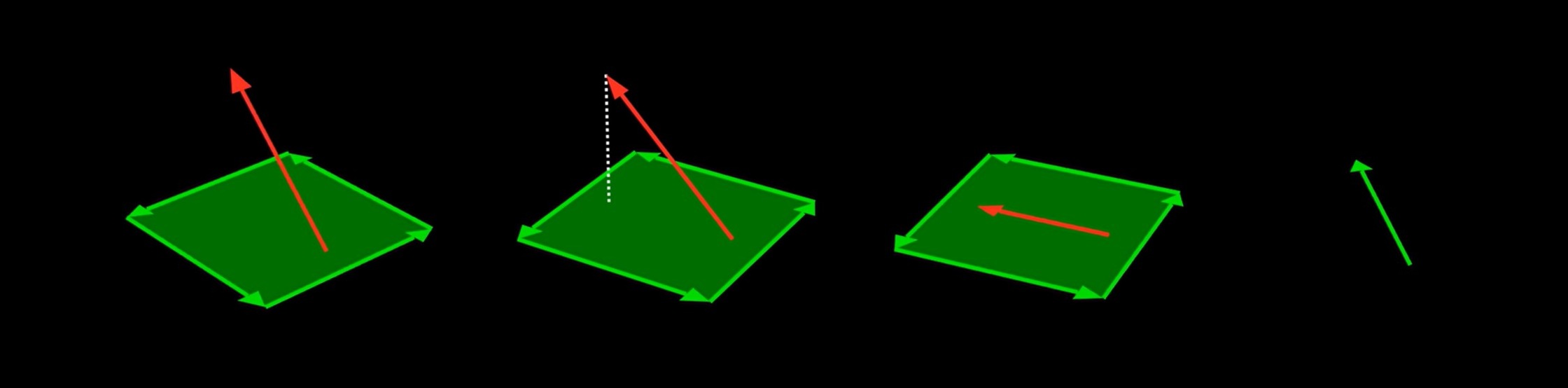
Dual
The dual in Geometric Algebra (GA) maps a multivector of grade \(k\) to a new multivector of grade \(n - k\) by multiplying it with the inverse of the unit pseudoscalar \(I^{-1}\). It is the algebraic equivalent of finding the orthogonal complement of a subspace, converting vectors to bivectors, and vice-versa.
The Mathematics of DualityThe duality operator, usually denoted by an asterisk (\({}^{*}\)) or a star (\(\star \)), essentially finds the perpendicular complement to a shape.
Dual
Orthogonal Complement
\( \text{Dual of } \color{red}{e_1} = \color{green}{e_{23}} \)
\( \text{Dual of } \color{red}{e_1} = -\color{green}{e_{23}}? \)
\( e_0^2 = 0 \)
\( \color{red}{e_1^2} = 1 \)
\( \color{red}{A}\color{green}{i} \)
\( = e_0\color{green}{i} \)
\( = e_0e_0\color{red}{e_1} \)
\( = 0 \)
Dual
\( \text{Dual of } A\text{: } \star A \)
\( \star A = Ai \)
\( A \star A = i \)
\( A \star A = |A|^2 i \)
\( A \star A = i \)
\( \text{When } A \text{ is normalized} \)
\( \text{Basis vectors: } \{e_1, e_2\} \)
\( \text{Basis multivectors: } \{1, e_1, e_2, e_{12}\} \)
\( 1 \star 1 = e_{12} \implies \star 1 = e_{12} \)
\( e_1 \star e_1 = e_{12} \implies \star e_1 = e_2 \)
\( e_2 \star e_2 = e_{12} \implies \star e_2 = -e_1 \)
\( e_{12} \star e_{12} = e_{12} \implies \star e_{12} = 1 \)
\( A \vee B = \star^{-1} (\star A \wedge \star B) \)
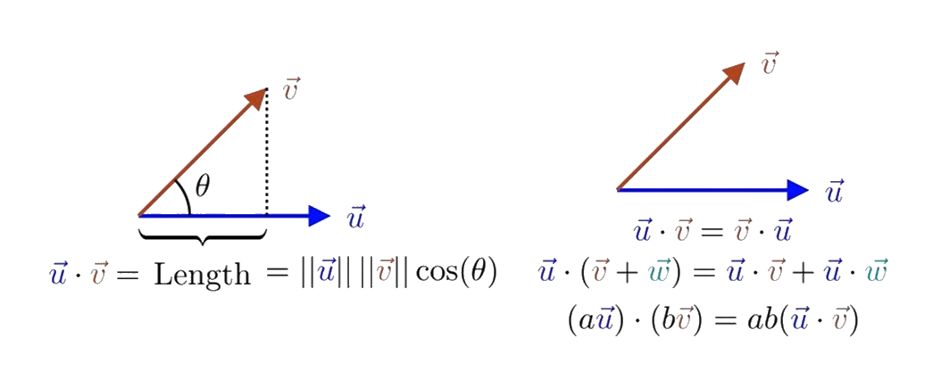
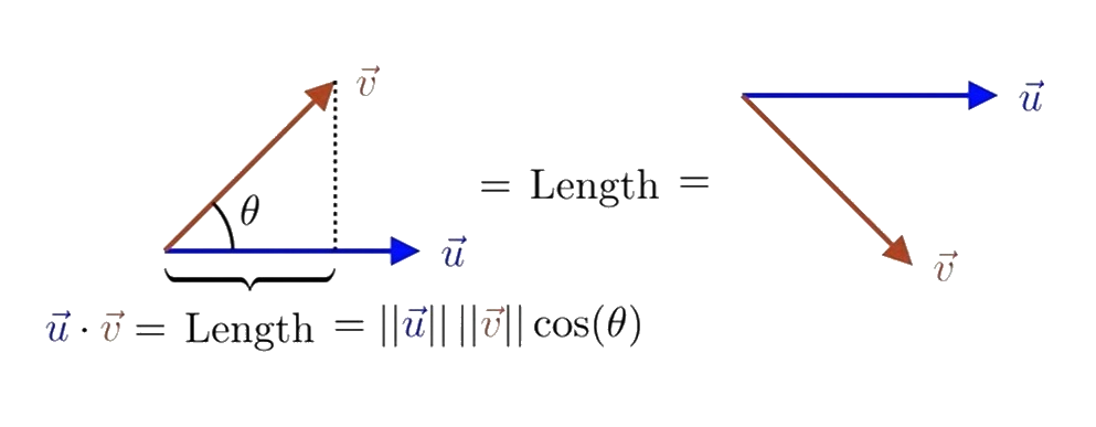
Inner Product
\(\text{Inner Product: A function that is bilinear, produces a scalar, is symmetric, and is positive definite.}\)
\(
\begin{array}{ll}
\\
\text{GA Inner Product:} & \bullet \text{ Bilinear} \\
& \bullet \text{ Produces a multivector} \\
& \bullet \text{ Not symmetric} \\
& \bullet \text{ Can produce negative scalars}
\end{array}
\)
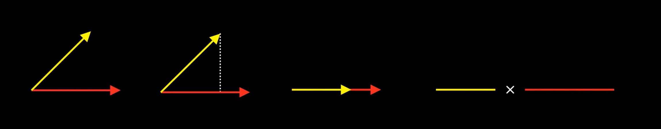
\( \text{Inner Product:} \quad \begin{aligned} &\text{Projection} + \text{Multiplication} \\ &\text{Projection} + \text{Contraction} \end{aligned} \)
\( \begin{aligned}
&A \cdot B \\
&\vec{a} \cdot \vec{B} \\\\
\text{Left Contraction:} \quad &A \rfloor B \\
\text{Right Contraction:} \quad &A \lfloor B \\
\text{Inner Product:} \quad &A \cdot B
\end{aligned} \)
\( \vec{a} \quad \vec{\vec{B}} \quad \vec{a}_{\parallel} = \text{Projection of } \vec{a} \text{ onto } \vec{\vec{B}} \)
\( \begin{aligned}
\vec{a} \rfloor \vec{\vec{B}} &= \vec{a}_{\parallel} \vec{\vec{B}} \\
\vec{a} \lfloor \vec{\vec{B}} &= 0 \\
\vec{a} \cdot \vec{\vec{B}} &= \vec{a}_{\parallel} \vec{\vec{B}} \\
\vec{\vec{B}} \rfloor \vec{a} &= 0 \\
\vec{\vec{B}} \lfloor \vec{a} &= \vec{\vec{B}} \vec{a}_{\parallel} \\
\vec{\vec{B}} \cdot \vec{a} &= \vec{\vec{B}} \vec{a}_{\parallel}
\end{aligned} \)
\( \begin{aligned}
&(e_{01} + e_{56}) \cdot (e_{1234} + e_{3456}) \\
& = e_{01} \cdot e_{1234} + e_{01} \cdot e_{3456} + e_{56} \cdot e_{1234} + e_{56} \cdot e_{3456} \\
& = e_{01} \cdot e_{1234} + e_{56} \cdot e_{3456} \\
& = e_{01} \cdot e_{1234} + e_{56} e_{3456} \\
& = e_{01} \cdot e_{1234} - e_{34} \\
& = -e_{34}
\end{aligned} \)
The outer product of two basis multivectors is their geometric product if they share no factors
The inner product of two basis multivectors is their geometric product if they share all factors
\( \begin{aligned}
A_j \wedge B_k &= \langle A_j B_k \rangle_{j+k} \\
A_j \rfloor B_k &= \langle A_j B_k \rangle_{k-j} \\
A_j \lfloor B_k &= \langle A_j B_k \rangle_{j-k} \\
A_j \cdot B_k &= \langle A_j B_k \rangle_{|j-k|}
\end{aligned} \)
When do we use the different inner products?
In applications: Use the inner product
In theory: Use the contractions
\( \begin{aligned}
\vec{a} B &\neq \vec{a} \cdot B + \vec{a} \wedge B \\
\vec{a} B &= \vec{a} \rfloor B + \vec{a} \wedge B \\
A B &\neq A \rfloor B + A \wedge B
\end{aligned} \)