


Laurent series
The Laurent series for a complex function \(f(z)\) about a point \(c\) is given by
\[f(z)={\textstyle\textstyle\mbox{$Σ$}_{n=-\infty}^\infty}{\textstyle a_n}{\textstyle{(z-c)}^n}\]
where \(a_n\) and \(c\) are constants, with \(a_n\) defined by a contour integral that generalizes Cauchy's integral formula:
\[{\textstyle{\scriptstyle a}_n}{\textstyle=}\frac1{2\mathrm{πi}}{\textstyle{\scriptstyle\oint}_\gamma}\frac{f(z)}{{(z-c)}^{n+1}}{\textstyle d}{\textstyle z}\]
Suppose that \(f(z)\) is analytic on the annulus
\[A: r_1 < |z - z_0| < r_2. \nonumber\]
Then \(f(z)\) can be expressed as a series
\[f(z) = \sum_{n = 1}^{\infty} \dfrac{b_n}{(z - z_0)^n} + \sum_{n = 0}^{\infty} a_n (z - z_0)^n. \nonumber\]
The coefficients have the formulus
\[\begin{array} {l} {a_n = \dfrac{1}{2\pi i} \int_{\gamma} \dfrac{f(w)}{(w - z_0)^{n + 1}}\ dw} \\ {b_n = \dfrac{1}{2\pi i} \int_{\gamma} f(w) (w - z_0)^{n - 1}\ dw} \end{array} \nonumber\]
where \(γ\) is any circle \(|w−z_0|=r\) inside the annulus, i.e. \(\;r_1<\;r\;<\;r_2 \)
Furthermore
The series \(\sum_{n = 0}^{\infty} a_n (z - z_0)^n\) converges to an analytic function for \(|z - z_0| < r_2\)
The series \(\sum_{n = 1}^{\infty} \dfrac{b_n}{(z - z_0)^n}\) converges to an analytic function for \(|z - z_0| > r_1\)
Together, the series both converge on the annulus \(A\) where \(f\) is analytic.
Conformal mapping

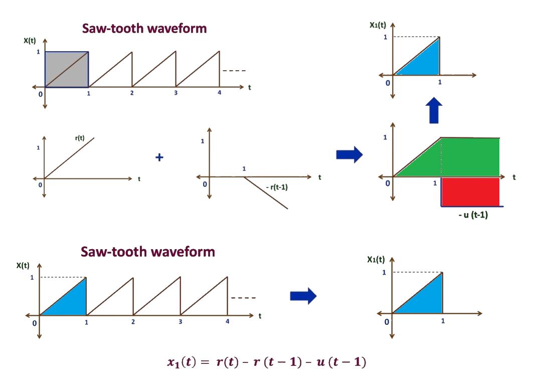
Signals and Systems
Signals ultilize "Fourier Transform"
Systems make use of "Laplace Transform"
Fourier transform time domain is \(from\;-\infty\;to\;\infty\)
Laplace transform time domain is \(from\;0^-\;to\;\infty\)
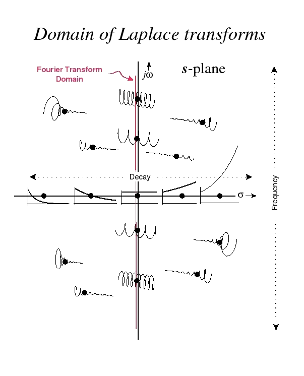
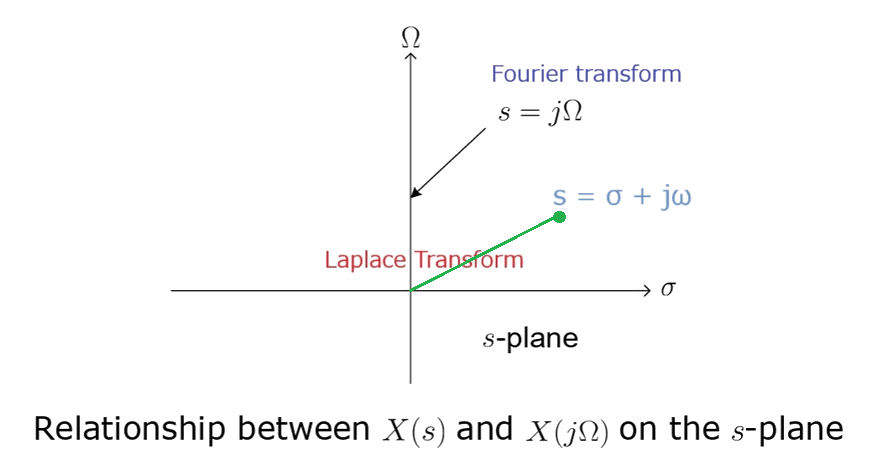
The Laplace transform converts a signal to a complex plane. The Fourier transform transforms the same signal into the jw plane and is a subset of the Laplace transform in which the real part is 0.
Discrete Fourier Transform - Represents the magnitude and phase of a discrete system.
Laplace Transforms - Represents the magnitude, phase, and dampening of a continuous system.
Z Transform - Represents the magnitude, phase, and dampening of a discrete system.
Laplace Transform
拉普拉斯轉換\(\mathcal F\{f(t)\}=\int_{-\infty}^\infty f(t)e^{-j\omega t}\operatorname dt=F(\omega)\)
\(\Rightarrow F(s)=\int_{-\infty}^\infty f(t)e^{-st}\operatorname dt\)
For practical signals, \(f(t),\;t\geq0\)
we define,
\(\mathcal L\{f(t)\}=F(s)\neq\int_0^\infty f(t)e^{-st}\operatorname dt\)
\(=\int_{0^-}^\infty f(t)e^{-st}\operatorname dt\)
\(s=\sigma+j\omega\)
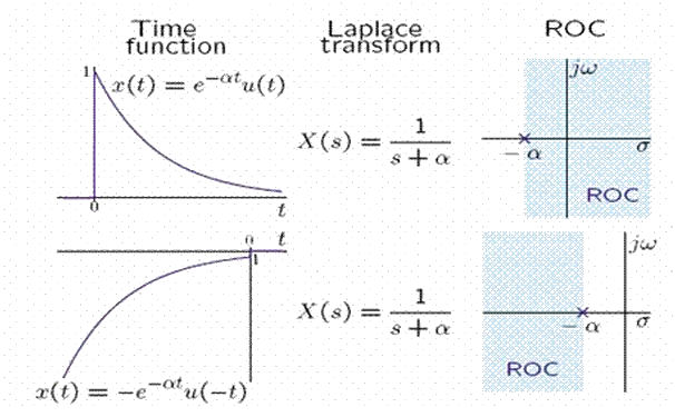
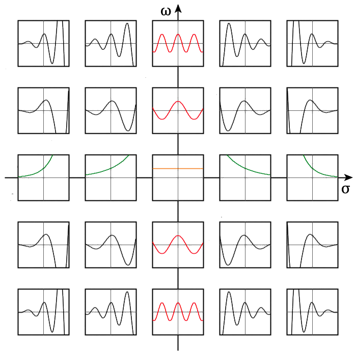
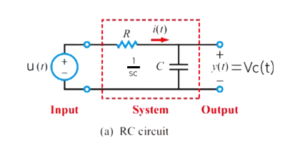
The Laplace transform is used where the Fourier transform cannot be used. The Laplace transform redefines the transform and includes an exponential convergence factor σ along with jω. Therefore, using the Laplace transform the time-domain signal x(t) can be represented as a sum of complex exponential functions of the form \(e^{st}\).
The advantage of using the Laplace transform is that it converts an ODE (Ordinary differential equation) into an algebraic equation of the same order that is simpler to solve, even though it is a function of a complex variable. The chapter discusses ways of solving ODEs using the phasor notation for sinusoidal signals.
In mathematics, the Laplace transform, named after its discoverer Pierre-Simon Laplace, is an integral transform that converts a function of a real variable (usually \(t\), in the time domain) to a function of a complex variable \(s\) (in the complex-valued frequency domain, also known as s-domain, or s-plane).
The Laplace transform is defined (for suitable functions \(f\)) by the integral:
\(ℒ\lbrack f(t)\rbrack=F(s) \overset{\rm{def}}{=} \int_{0^-}^{\infty} e^{-st}f(t)\,dt. \nonumber\)
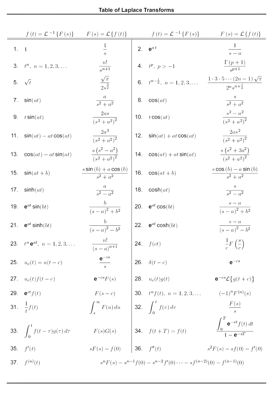
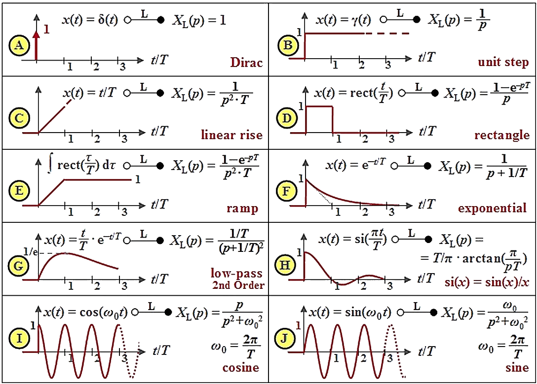
Table of Laplace Transforms
| \(f\left( t \right) = {\mathcal{L}^{\,\, - 1}}\left\{ {F\left( s \right)} \right\}\) | \(F\left( s \right) = \mathcal{L}\left\{ {f\left( t \right)} \right\}\) | |
|---|---|---|
| 1. | 1 | \(\displaystyle \frac{1}{s}\) |
| 2. | \({{\bf{e}}^{a\,t}}\) | \(\displaystyle \frac{1}{{s - a}}\) |
| 3. | \({t^n},\,\,\,\,\,n = 1,2,3, \ldots \) | \(\displaystyle \frac{{n!}}{{{s^{n + 1}}}}\) |
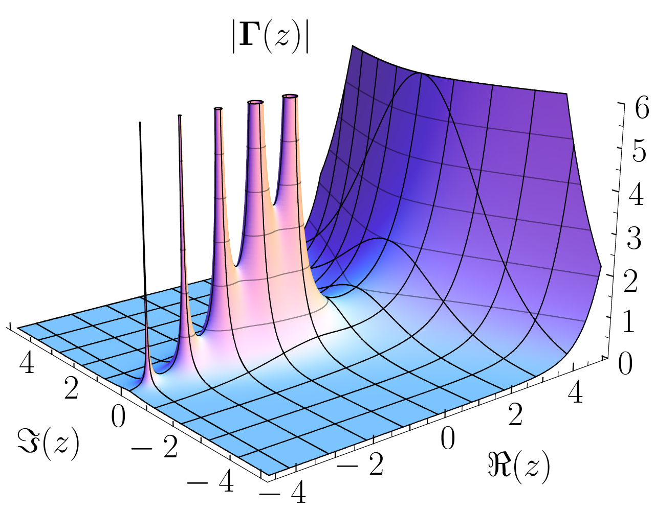
| 4. | \({t^p}\), \(p > -1\) | \(\displaystyle \frac{{\Gamma \left( {p + 1} \right)}}{{{s^{p + 1}}}}\) |
| 5. | \(\sqrt t \) | \(\displaystyle \frac{{\sqrt \pi }}{{2{s^{\frac{3}{2}}}}}\) |
| 6. | \({t^{n - \frac{1}{2}}},\,\,\,\,\,n = 1,2,3, \ldots \) | \(\displaystyle \frac{{1 \cdot 3 \cdot 5 \cdots \left( {2n - 1} \right)\sqrt \pi }}{{{2^n}{s^{n + \frac{1}{2}}}}}\) |
| 7. | \(\sin \left( {at} \right)\) | \(\displaystyle \frac{a}{{{s^2} + {a^2}}}\) |
| 8. | \(\cos \left( {at} \right)\) | \(\displaystyle \frac{s}{{{s^2} + {a^2}}}\) |
| 9. | \(t\sin \left( {at} \right)\) | \(\displaystyle \frac{{2as}}{{{{\left( {{s^2} + {a^2}} \right)}^2}}}\) |
| 10. | \(t\cos \left( {at} \right)\) | \(\displaystyle \frac{{{s^2} - {a^2}}}{{{{\left( {{s^2} + {a^2}} \right)}^2}}}\) |
| 11. | \(\sin \left( {at} \right) - at\cos \left( {at} \right)\) | \(\displaystyle \frac{{2{a^3}}}{{{{\left( {{s^2} + {a^2}} \right)}^2}}}\) |
| 12. | \(\sin \left( {at} \right) + at\cos \left( {at} \right)\) | \(\displaystyle \frac{{2a{s^2}}}{{{{\left( {{s^2} + {a^2}} \right)}^2}}}\) |
| 13. | \(\cos \left( {at} \right) - at\sin \left( {at} \right)\) | \(\displaystyle \frac{{s\left( {{s^2} - {a^2}} \right)}}{{{{\left( {{s^2} + {a^2}} \right)}^2}}}\) |
| 14. | \(\cos \left( {at} \right) + at\sin \left( {at} \right)\) | \(\displaystyle \frac{{s\left( {{s^2} + 3{a^2}} \right)}}{{{{\left( {{s^2} + {a^2}} \right)}^2}}}\) |
| 15. | \(\sin \left( {at + b} \right)\) | \(\displaystyle \frac{{s\sin \left( b \right) + a\cos \left( b \right)}}{{{s^2} + {a^2}}}\) |
| 16. | \(\cos \left( {at + b} \right)\) | \(\displaystyle \frac{{s\cos \left( b \right) - a\sin \left( b \right)}}{{{s^2} + {a^2}}}\) |
| 17. | \(\sinh \left( {at} \right)\) | \(\displaystyle \frac{a}{{{s^2} - {a^2}}}\) |
| 18. | \(\cosh \left( {at} \right)\) | \(\displaystyle \frac{s}{{{s^2} - {a^2}}}\) |
| 19. | \({{\bf{e}}^{at}}\sin \left( {bt} \right)\) | \(\displaystyle \frac{b}{{{{\left( {s - a} \right)}^2} + {b^2}}}\) |
| 20. | \({{\bf{e}}^{at}}\cos \left( {bt} \right)\) | \(\displaystyle \frac{{s - a}}{{{{\left( {s - a} \right)}^2} + {b^2}}}\) |
| 21. | \({{\bf{e}}^{at}}\sinh \left( {bt} \right)\) | \(\displaystyle \frac{b}{{{{\left( {s - a} \right)}^2} - {b^2}}}\) |
| 22. | \({{\bf{e}}^{at}}\cosh \left( {bt} \right)\) | \(\displaystyle \frac{{s - a}}{{{{\left( {s - a} \right)}^2} - {b^2}}}\) |
| 23. | \({t^n}{{\bf{e}}^{at}},\,\,\,\,\,n = 1,2,3, \ldots \) | \(\displaystyle \frac{{n!}}{{{{\left( {s - a} \right)}^{n + 1}}}}\) |
| 24. | \(f\left( {ct} \right)\) | \(\displaystyle \frac{1}{c}F\left( {\frac{s}{c}} \right)\) |
| 25. | \({u_c}\left( t \right) = u\left( {t - c} \right)\) | \(\displaystyle \frac{{{{\bf{e}}^{ - cs}}}}{s}\) |
| 26. | \(\delta \left( {t - c} \right)\) | \({{\bf{e}}^{ - cs}}\) |
| 27. | \({u_c}\left( t \right)f\left( {t - c} \right)\) | \({{\bf{e}}^{ - cs}}F\left( s \right)\) |
| 28. | \({u_c}\left( t \right)g\left( t \right)\) | \({{\bf{e}}^{ - cs}}{\mathcal{L}}\left\{ {g\left( {t + c} \right)} \right\}\) |
| 29. | \({{\bf{e}}^{ct}}f\left( t \right)\) | \(F\left( {s - c} \right)\) |
| 30. | \({t^n}f\left( t \right),\,\,\,\,\,n = 1,2,3, \ldots \) | \({\left( { - 1} \right)^n}{F^{\left( n \right)}}\left( s \right)\) |
| 31. | \(\displaystyle \frac{1}{t}f\left( t \right)\) | \(\int_{{\,s}}^{{\,\infty }}{{F\left( u \right)\,du}}\) |
| 32. | \(\displaystyle \int_{{\,0}}^{{\,t}}{{\,f\left( v \right)\,dv}}\) | \(\displaystyle \frac{{F\left( s \right)}}{s}\) |
| 33. | \(\displaystyle \int_{{\,0}}^{{\,t}}{{f\left( {t - \tau } \right)g\left( \tau \right)\,d\tau }}\) | \(F\left( s \right)G\left( s \right)\) |
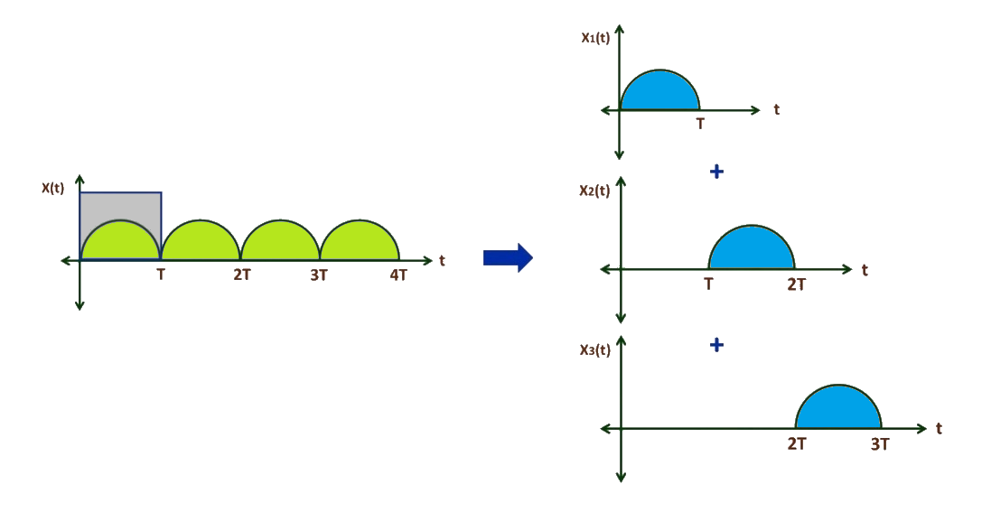
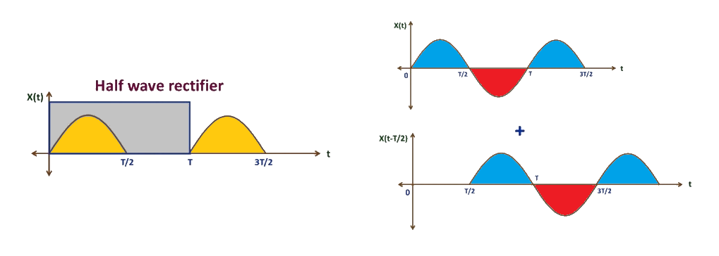
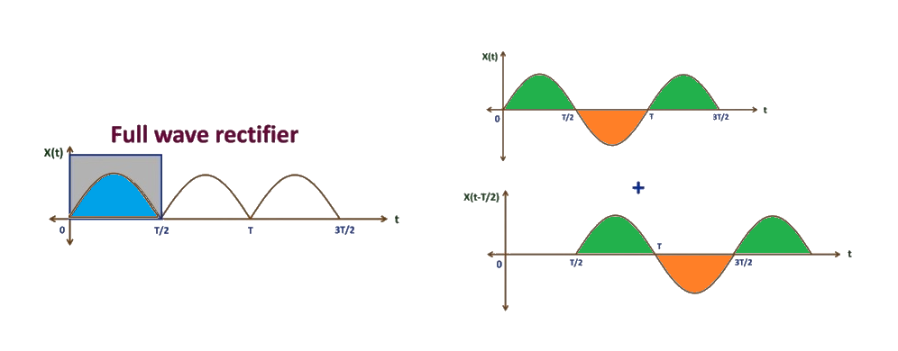
| 34. | \(f\left( {t + T} \right) = f\left( t \right)\) | \(\displaystyle \frac{{\displaystyle \int_{{\,0}}^{{\,T}}{{{{\bf{e}}^{ - st}}f\left( t \right)\,dt}}}}{{1 - {{\bf{e}}^{ - sT}}}}\) |
| 35. | \(f'\left( t \right)\) | \(sF\left( s \right) - f\left( 0 \right)\) |
| 36. | \(f''\left( t \right)\) | \({s^2}F\left( s \right) - sf\left( 0 \right) - f'\left( 0 \right)\) |
| 37. | \({f^{\left( n \right)}}\left( t \right)\) | \({s^n}F\left( s \right) - {s^{n - 1}}f\left( 0 \right) - {s^{n - 2}}f'\left( 0 \right) \cdots - s{f^{\left( {n - 2} \right)}}\left( 0 \right) - {f^{\left( {n - 1} \right)}}\left( 0 \right)\) |