


Mathematics Yoshio Mar 24th, 2024 at 8:00 PM 8 0
線性代數
Linear AlgebraIn math terms, an operation F is linear if scaling inputs scales the output, and adding inputs adds the outputs:
\(F(\alpha\overset\rightharpoonup x)=\alpha\cdot F(\overset\rightharpoonup x)\)
\(F(\overset\rightharpoonup x+\overset\rightharpoonup y)=F(\overset\rightharpoonup x)+F(\overset\rightharpoonup y)\)
[Ex] \(x{\color[rgb]{0.0, 0.0, 1.0}C}_{\color[rgb]{0.0, 0.0, 1.0}2}{\color[rgb]{0.0, 0.0, 1.0}H}_{\color[rgb]{0.0, 0.0, 1.0}5}{\color[rgb]{0.0, 0.0, 1.0}O}{\color[rgb]{0.0, 0.0, 1.0}H}+y{\color[rgb]{0.0, 0.0, 1.0}O}_{\color[rgb]{0.0, 0.0, 1.0}2}\Rightarrow z{\color[rgb]{0.0, 0.0, 1.0}C}{\color[rgb]{0.0, 0.0, 1.0}O}_{\color[rgb]{0.0, 0.0, 1.0}2}+w{\color[rgb]{0.0, 0.0, 1.0}H}_{\color[rgb]{0.0, 0.0, 1.0}2}{\color[rgb]{0.0, 0.0, 1.0}O}\)
\(x{\color[rgb]{0.0, 0.0, 1.0}\begin{bmatrix}2\\1\\6\end{bmatrix}}+y{\color[rgb]{0.0, 0.0, 1.0}\begin{bmatrix}{\color[rgb]{0.0, 0.0, 0.0}0}\\2\\{\color[rgb]{0.0, 0.0, 0.0}0}\end{bmatrix}}=z{\color[rgb]{0.0, 0.0, 1.0}\begin{bmatrix}1\\2\\{\color[rgb]{0.0, 0.0, 0.0}0}\end{bmatrix}}+w{\color[rgb]{0.0, 0.0, 1.0}\begin{bmatrix}{\color[rgb]{0.0, 0.0, 0.0}0}\\1\\2\end{bmatrix}}\)
\({\color[rgb]{0.0, 0.0, 1.0}\begin{bmatrix}2&{\color[rgb]{0.1, 0.1, 0.1}0}&-1&{\color[rgb]{0.1, 0.1, 0.1}-}{\color[rgb]{0.1, 0.1, 0.1}0}\\1&2&-2&-1\\6&{\color[rgb]{0.1, 0.1, 0.1}0}&{\color[rgb]{0.1, 0.1, 0.1}-}{\color[rgb]{0.1, 0.1, 0.1}0}&-2\end{bmatrix}}\begin{bmatrix}x\\y\\z\\w\end{bmatrix}={\color[rgb]{1.0, 0.0, 0.0}\begin{bmatrix}0\\0\\0\end{bmatrix}}\)
[Ex] \(xSeCl_6+yO_2\rightarrow zSeO_2+tCl_2\)
\(\begin{bmatrix}\#Se\\\#Cl\\\#O\end{bmatrix}\;\;\;\;x\begin{bmatrix}1\\6\\0\end{bmatrix}+y\begin{bmatrix}0\\0\\2\end{bmatrix}=z\begin{bmatrix}1\\0\\2\end{bmatrix}+t\begin{bmatrix}0\\2\\0\end{bmatrix}\)
\(x\begin{bmatrix}1\\6\\0\end{bmatrix}+y\begin{bmatrix}0\\0\\2\end{bmatrix}-z\begin{bmatrix}1\\0\\2\end{bmatrix}-t\begin{bmatrix}0\\2\\0\end{bmatrix}=\begin{bmatrix}0\\0\\0\end{bmatrix}\)
\(\begin{bmatrix}1&0&-1&0\\6&0&0&-2\\0&2&-2&0\end{bmatrix}\begin{bmatrix}x\\y\\z\\t\end{bmatrix}=\begin{bmatrix}0\\0\\0\end{bmatrix}\)
Find the null space, \(\begin{bmatrix}1&0&0&-\frac13\\0&1&0&-\frac13\\0&0&1&-\frac13\end{bmatrix}\)
\(\overline x=\begin{bmatrix}1&1&1&3\end{bmatrix}^T\)
\(\therefore SeCl_6+O_2\rightarrow SeO_2+3Cl_2\)
The null space's insight into chemical balance
The ability to take a combination of substances and tally the amounts of each element is a key part of the balancing process.
The combustion of ethylene has one solution
\({{\mathrm C}_2{\mathrm H}_4}+{\mathrm O}_2\leftrightarrow{\mathrm C\mathrm O}_2+{{\mathrm H}_2\mathrm O}\)
\(\begin{pmatrix}&C_2H_4&O_2&CO_2&H_2O\\C&2&0&1&0\\H&4&0&0&2\\O&0&2&2&1\end{pmatrix}\)
transpose \(\begin{bmatrix}2&4&0\\0&0&2\\1&0&2\\0&2&1\end{bmatrix}\)
\(\left|{\begin{array}{ccc|cccc}2&4&0&1&0&0&0\\0&0&2&0&1&0&0\\1&0&2&0&0&1&0\\0&2&1&0&0&0&1\end{array}}\right|\)
\(rref\;{\left|{\begin{array}{ccc|cccc}2&4&0&1&0&0&0\\0&0&2&0&1&0&0\\1&0&2&0&0&1&0\\0&2&1&0&0&0&1\end{array}}\right|}={\left|{\begin{array}{ccc|cccc}1&0&0&0&-1&1&0\\0&1&0&0&-1/4&0&1/2\\0&0&1&0&1/2&0&0\\0&0&0&1&3&-2&-2\end{array}}\right|}\)
We examine the row echelon form's left side for rows of all zero. Here, there's exactly one— the last row:
\({\lbrack\begin{array}{ccc|cccc}0&0&0&1&3&-2&-2\end{array}\rbrack}.\)
\(1⋅{\mathrm C}_2{\mathrm H}_4+3⋅{\mathrm O}_2\leftrightarrow2⋅\mathrm C{\mathrm O}_2+2⋅{\mathrm H}_2\mathrm O.\)
\({\mathrm C}_2{\mathrm H}_4+3{\mathrm O}_2\leftrightarrow2{\mathrm{CO}}_2+2{\mathrm H}_2\mathrm O\)
We can balance electric charge, too
\(\mathrm H^++\mathrm C{\mathrm r}_2\mathrm O_7^{2-}+{\mathrm C}_2{\mathrm H}_5\mathrm O\mathrm H\leftrightarrow\mathrm C\mathrm r^{3+}+\mathrm C{\mathrm O}_2+{\mathrm H}_2\mathrm O.\)
\(\begin{bmatrix}1&0&6&0&0&2\\0&2&0&1&0&0\\0&7&1&0&2&1\\0&0&2&0&1&0\\+1&-2&0&+3&0&0\end{bmatrix}\)
\({\left|{\begin{array}{ccccc|cccccc}1&0&0&0&+1&1&0&0&0&0&0\\0&2&7&0&-2&0&1&0&0&0&0\\6&0&1&2&0&0&0&1&0&0&0\\0&1&0&0&+3&0&0&0&1&0&0\\0&0&2&1&0&0&0&0&0&1&0\\2&0&1&0&0&0&0&0&0&0&1\end{array}}\right|}.\)
\({\lbrack\begin{array}{ccccc|cccccc}0&0&0&0&0&1&1/8&1/16&-1/4&-1/8&-11/16\end{array}\rbrack}.\)
\({\lbrack\begin{array}{ccccc|cccccc}0&0&0&0&0&16&2&1&-4&-2&-11\end{array}\rbrack}.\)
\(16{}\mathrm H^++2{}\mathrm C{\mathrm r}_2\mathrm O_7^{2-}+{\mathrm C}_2{\mathrm H}_5\mathrm O\mathrm H\leftrightarrow4{}\mathrm C\mathrm r^{3+}+2{}\mathrm C{\mathrm O}_2+11{}{\mathrm H}_2\mathrm O.\)
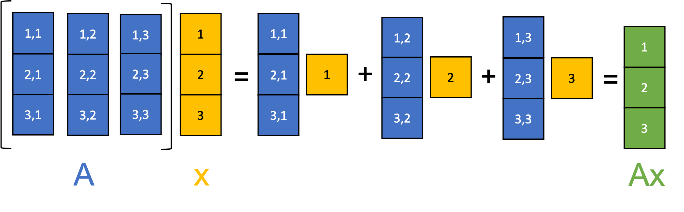

Linear algebra provides an invaluable tool kit for computation tasks such as solving a system of linear equations or finding the inverse of a square matrix. Given that these tasks usually involve a large number of calculations, it is often the case that the geometric interpretation is underappreciated. Linear algebra is a genuine oddity in that it is possible to understand this entire discipline with multiple, distinct perspectives, each of which has its own merits and its own way of understanding this vast and elegant subject. A criminally overlooked perspective for new students of linear algebra is the one in which we think of matrices as a way of transforming vectors, hence offering us a well-developed tool kit to start describing (linear) spatial geometry.
Vectors are special types of matrices which can be split into two categories: row vectors and column vectors. A row vector is a matrix of order \(1\times n\), which has \(1\) row and \(n\) columns, whereas a column vector is a matrix of order \(m\times1\) which has \(m\) rows and \(1\) column. Although convention differs from source to source, it is arguably most sensible to think only in terms of column vectors. There are two reasons for this: column vectors are used more often and can be related to row vectors by transposition if needed; and column vectors are possible to combine with matrices under matrix multiplication on the left-hand side (which is also simply a matter of arbitrary convention but for some reason it just feels better).
\(a=\begin{pmatrix}3\\2\end{pmatrix},\;b=\begin{pmatrix}-5\\2\end{pmatrix}\)

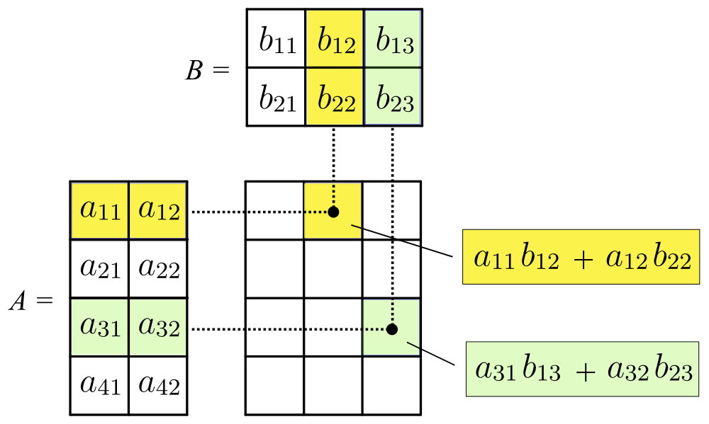
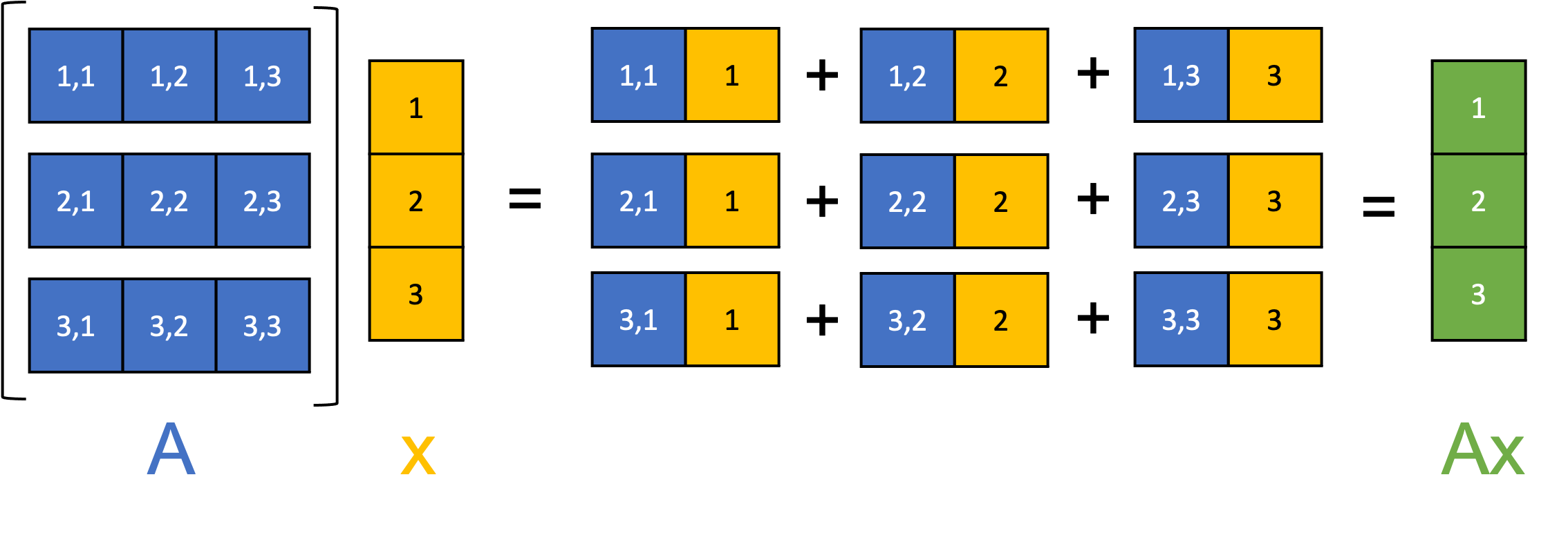
The matrix multiplication \(AB\) is well defined so long as \(A\) has order \(m\times n\) and \(B\) has order \(n\times p\) The resulting matrix is of order \(m\times p\).
uppose now that we were to consider the matrix products \(a'=Ma\) and \(b'=Mb\).
\(M=\begin{pmatrix}1&2\\-1&3\end{pmatrix}\)
\(a'=Ma=\begin{pmatrix}1&2\\-1&3\end{pmatrix}\begin{pmatrix}3\\2\end{pmatrix}=\begin{pmatrix}7\\3\end{pmatrix}\)
\(b'=Mb=\begin{pmatrix}1&2\\-1&3\end{pmatrix}\begin{pmatrix}-5\\2\end{pmatrix}=\begin{pmatrix}-1\\11\end{pmatrix}\)

\(M=\begin{pmatrix}2&-1\\1&1\end{pmatrix}\)
\(a'=Ma=\begin{pmatrix}2&-1\\1&1\end{pmatrix}\begin{pmatrix}3\\2\end{pmatrix}=\begin{pmatrix}4\\5\end{pmatrix}\)
\(b'=Mb=\begin{pmatrix}2&-1\\1&1\end{pmatrix}\begin{pmatrix}-5\\2\end{pmatrix}=\begin{pmatrix}-12\\-3\end{pmatrix}\)

Eigenvalues and Eigenvectors
The prefix eigen- is adopted from the German word eigen (cognate with the English word own) for 'proper', 'characteristic', 'own'.
\(A \vec{v} =\lambda \vec{v} \)
Notice we multiply a squarematrix by a vector and get the same result as when we multiply a scalar (just a number) by that vector.
We start by finding the eigenvalue. We know this equation must be true:
\(A \vec{v} =\lambda \vec{v} \)
Next we put in an identity matrix so we are dealing with matrix-vs-matrix:
\(A \vec{v} =\lambda {I} \vec{v} \)
Bring all to left hand side:
\(A \vec{v} -\lambda I \vec{v} = 0\)
If v is non-zero then we can (hopefully) solve for λ using just the determinant:
\(det(A - \lambda I) = 0\)
\(| A − \lambda I | = 0\)
trace of A
The matrix A has n eigenvalues (including each according to its multiplicity). The sum of the n eigenvalues of A is the same as the trace of A (that is, the sum of the diagonal elements of A). The product of the n eigenvalues of A is the same as the determinant of A.

Perpendicular Vector
While both involve multiplying the magnitudes of two vectors, the dot product results in a scalar quantity, which indicates magnitude but not direction, while the cross product results in a vector, which indicates magnitude and direction.
Inner product (Dot product)
Since the inner product generalizes the dot product, it is reasonable to say that two vectors are “orthogonal” (or “perpendicular”) if their inner product is zero. With this definition, we see from the preceding example that sin x and cosx are orthogonal (on the interval [−π, π]).
\(\overset\rightharpoonup A\cdot\overset\rightharpoonup B=\sum_{i=1}^n\;a_ib_i=a_1b_1+a_2b_2+\cdots+a_nb_n\)
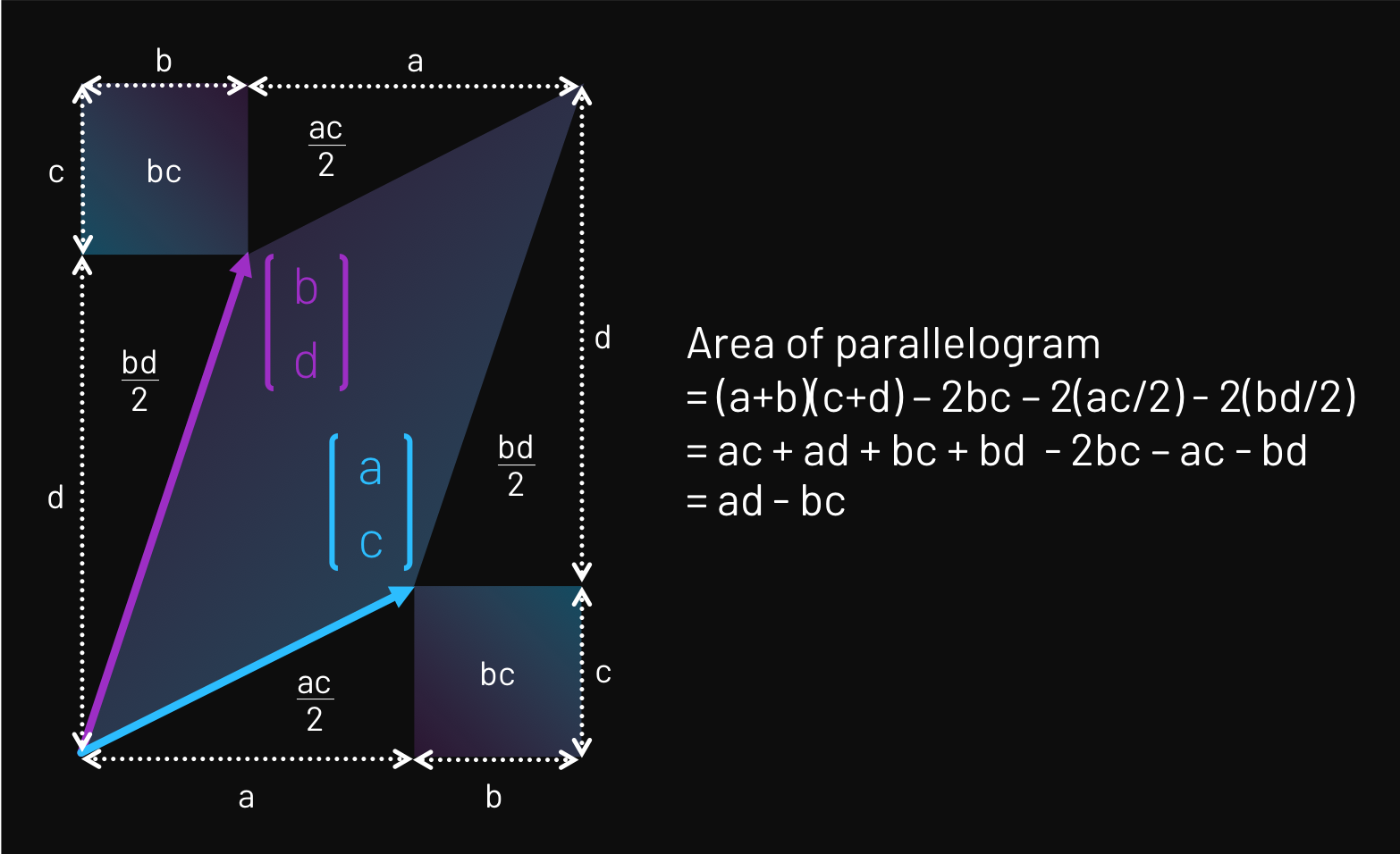
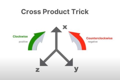
Outer product (Cross product)
A cross product of any two vectors yields a vector which is perpendicular to both vectors .
\(\because\) for two vectors \(\overrightarrow A\) and \(\overrightarrow B\), if \(\overrightarrow C\) is the vector perpendicular to both.
\(\overrightarrow C=\overrightarrow A\times\overrightarrow B=\begin{bmatrix}\widehat i&\widehat j&\widehat k\\A_1&A_2&A_3\\B_1&B_2&B_3\end{bmatrix}\\=(A_2B_3-B_2A_3)\widehat i-(A_1B_3-B_1A_3)\widehat j+(A_1B_2-B_1A_2)\widehat k\)
Inserting given vectors we obtain
\(\overrightarrow C=\begin{bmatrix}\widehat i&\widehat j&\widehat k\\2&3&4\\1&2&3\end{bmatrix}\)
\(={(3\times3-2\times4)}\widehat i-{(2\times3-1\times4)}\widehat j+{(2\times2-1\times3)}\widehat k\)
\(=\widehat i-2\widehat j+\widehat k\)
Cross product trick
\( \vec{A} \times \vec{B}=\begin{vmatrix} \hat{i}&\hat{j}&\hat{k} \\ A_x & A_y & A_z \\ B_x&B_y&B_z \end{vmatrix} \)
\( \vec{A}\times\vec{B}=(A_y B_z- A_z B_y)\hat{i}+(A_z B_x - A_x B_z) \hat{j}+(A_x B_y- A_y B_x) \hat{k} \nonumber \)
Matrix multiplication
There are two basic types of matrix multiplication: inner (dot) product and outer product. The inner product results in a matrix of reduced dimensions, the outer product results in one of expanded dimensions. A helpful mnemonic: Expand outward, contract inward.
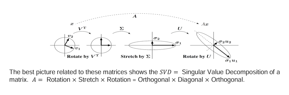
Eigenvalue Decomposition
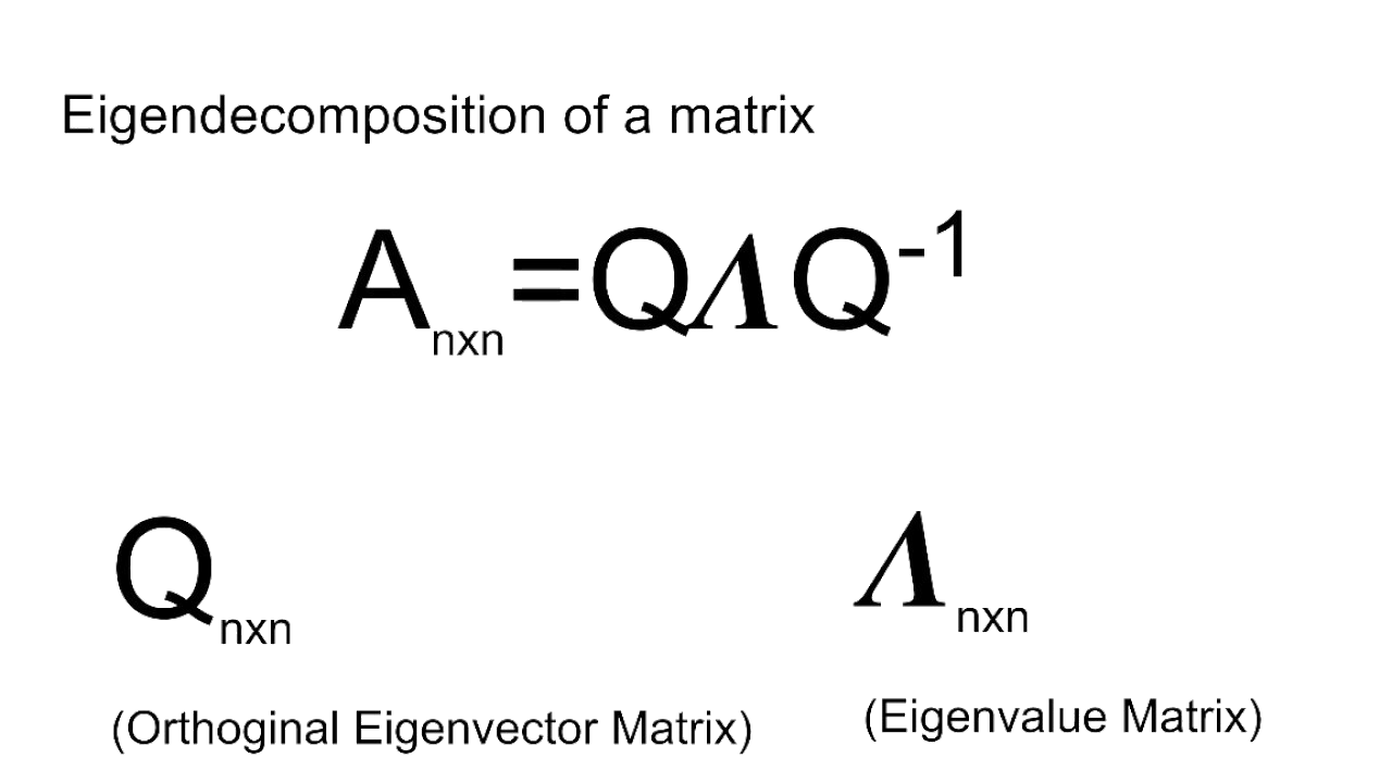

\[\begin{bmatrix}\mathtt{\,\,\,\,0}&\mathtt{\,\,\,\,1}\\\mathtt{-2}&\mathtt{-3}\end{bmatrix}\begin{bmatrix}\mathtt{-1}&\mathtt{-1}\\\mathtt{\,\,\,\,2}&\mathtt{\,\,\,\,1}\end{bmatrix}=\begin{bmatrix}\mathtt{-1}&\mathtt{-1}\\\mathtt{\,\,\,\,2}&\mathtt{\,\,\,\,1}\end{bmatrix}\begin{bmatrix}\mathtt{-2}&\mathtt{\,\,\,\,0}\\\mathtt{\,\,\,\,0}&\mathtt{-1}\end{bmatrix}\]
\[\begin{bmatrix}\mathtt{\,\,\,\,0}&\mathtt{\,\,\,\,1}\\\mathtt{-2}&\mathtt{-3}\end{bmatrix}=\begin{bmatrix}\mathtt{-1}&\mathtt{-1}\\\mathtt{\,\,\,\,2}&\mathtt{\,\,\,\,1}\end{bmatrix}\begin{bmatrix}\mathtt{-2}&\mathtt{\,\,\,\,0}\\\mathtt{\,\,\,\,0}&\mathtt{-1}\end{bmatrix}\begin{bmatrix}\mathtt{\,\,\,\,1}&\mathtt{\,\,\,\,1}\\\mathtt{-2}&\mathtt{-1}\end{bmatrix}\]
Example (A)
As a real example of this, consider a simple model of the weather. Let’s say it either is sunny or it rains. If it’s sunny, there’s a 90% chance that it remains sunny, and a 10% chance that it rains the next day. If it rains, there’s a 40% chance it rains the next day, but a 60% chance of becoming sunny the next day. We can describe the time evolution of this process through a matrix equation:
\( \begin{bmatrix}{}_{Ps,n+1}\\{}_{Pr,n+1}\end{bmatrix}=\begin{bmatrix}0.9&0.6\\0.1&0.4\end{bmatrix}\begin{bmatrix}{}_{Ps,n}\\{}_{Pr,n}\end{bmatrix} \)
where \({}_{Ps,n}\), \({}_{Ps,n}\) are the probabilities that it is sunny or that it rains on day \(n\). (If you are curious, this kind of process is called a Markov process, and the matrix that I
have defined is called the transition matrix. This is, by the way, not a very good model of the weather.) One way to see that this matrix does provide the intended result is to see what results from
matrix multiplication:
\(p_{s,n+1}=0.9p_{s,n}+0.6p_{r,n}\)
\(p_{r,n+1}=0.1p_{s,n}+0.4p_{r,n}\)
This is just the law of total probability! To get a sense of the long run probabilities of whether it rains or not, let’s look at the eigenvectors and eigenvalues.
\(\begin{bmatrix}0.986394\\0.164399\end{bmatrix}\) with eigenvalue 1, \(\begin{bmatrix}‐0.707\\0.707\end{bmatrix}\) with eigenvalue 0.3
Now, this matrix ends up having an eigenvector of eigenvalue 1 (in fact, all valid Markov transition matrices do), while the other eigenvector is both unphysical (probabilities cannot be negative) and
has an eigenvalue less than 1. Therefore, in the long run, we expect the probability of it being sunny to be 0.986 and the probability of it being rainy to be 0.164 in this model.
This is known as the stationary distribution. Any component of the vector in the direction of the unphysical eigenvector will wither away in the long run (its eigenvalue is 0.3, and
\(0.3^k\rightarrow0\;as\;k\rightarrow\infty\), while the one with eigenvalue 1 will survive and dominate.
Eigenspaces
The set of all eigenvectors of T corresponding to the same eigenvalue, together with the zero vector, is called an eigenspace, or the characteristic space of T associated with that eigenvalue. If a set of eigenvectors of T forms a basis of the domain of T, then this basis is called an eigenbasis.
Eigenvectors of Symmetric Matrices Are Orthogonal
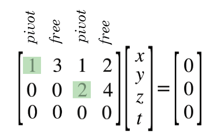
軸元 Pivot
軸元(英語:pivot或pivot element)是矩陣、陣列或是其他有限集合的一個演算元素,算法(如高斯消去法、快速排序、單體法等等)首先選出軸元,用於特定計算。
The pivot or pivot element is the element of a matrix, or an array, which is selected first by an algorithm (e.g. Gaussian elimination, simplex algorithm, etc.), to do certain calculations.

Markov chain
A Markov chain or Markov process is a stochastic model describing a sequence of possible events in which the probability of each event depends only on the state attained in the previous event. Informally, this may be thought of as, "What happens next depends only on the state of affairs now." A countably infinite sequence, in which the chain moves state at discrete time steps, gives a discrete-time Markov chain (DTMC). A continuous-time process is called a continuous-time Markov chain (CTMC). It is named after the Russian mathematician Andrey Markov.
Markov chains have many applications as statistical models of real-world processes, such as studying cruise control systems in motor vehicles, queues or lines of customers arriving at an airport, currency exchange rates and animal population dynamics.

Example (B)
The Linear Algebra View of the Fibonacci Sequence

The Fibonacci sequence first appears in the book Liber Abaci (The Book of Calculation, 1202) by Fibonacci where it is used to calculate the growth of rabbit populations.
0, 1, 1, 2, 3, 5, 8, 13, 21, 34, 55, 89, 144, ....
Each term in the Fibonacci sequence equals the sum of the previous two. That is, if we let Fn denote the nth term in the sequence we can write
\(F_n=F_{n-1}+F_{n-2}\)
To make this into a linear system, we need at least one more equation. Let’s use an easy one:
\(F_{n-1}=F_{n-1}+\left(0\right)\times F_{n-2}\)
Putting these together, here’s our system of linear equations for the Fibonacci sequence:
\(F_n=F_{n-1}+F_{n-2}\)
\(F_{n-1}=F_{n-1}+0\)
We can write this in matrix notation as the following:
\(\begin{bmatrix}F_n\\F_{n-1}\end{bmatrix}=\begin{bmatrix}1&1\\1&0\end{bmatrix}\begin{bmatrix}F_{n-1}\\F_{n-2}\end{bmatrix}\)
Here’s how we do that:
\(\begin{vmatrix}1-\lambda&1\\1&-\lambda\end{vmatrix}=0\)
\((1-\lambda)(-\lambda)-1=0\)
\(\lambda^2-\lambda-1=0\)
get the following two solutions, which are our two eigenvalues:
\(\lambda_1=\frac{1+\sqrt5}2\)
\(\lambda_2=\frac{1-\sqrt5}2\)
The next step is to find the two eigenvectors that correspond to the eigenvalues.
\(\left(A-\lambda I\right)x=0\)
we have the eigenvalues and eigenvectors, we can write the \(\mathrm S\) and \(\Lambda\) matrices as follows:
\(\mathrm S=\begin{bmatrix}\frac{1+\sqrt5}2&\frac{1-\sqrt5}2\\1&1\end{bmatrix}\)
\(\mathrm\Lambda=\begin{bmatrix}\frac{1+\sqrt5}2&0\\0&\frac{1-\sqrt5}2\end{bmatrix}\)
\(\mathrm S^{-1}=\frac1{\sqrt5}\begin{bmatrix}1&\frac{\sqrt5-1}2\\-1&\frac{\sqrt{5+1}}2\end{bmatrix}=\begin{bmatrix}\frac1{\sqrt5}&\frac{\sqrt5-1}{2\sqrt5}\\-\frac1{\sqrt5}&\frac{\sqrt{5+1}}{2\sqrt5}\end{bmatrix}\)
\({38}_{th}=39088169\), and \({39}_{th}\) is ?
\(39088169\times\frac{1+\sqrt5}2=39088169\times1.61803398875=63245986\)
\(39088169\div\frac{1-\sqrt5}2=39088169\div-0.61803398875=-63245986\),
\(\left|-63245986\right|=63245986\)
\({57}_{th}=365435296162\), and \({56}_{th}\) is ?
\(365435296162\div\frac{1+\sqrt5}2=365435296162\div1.61803398875=225851433717\)
\(365435296162\times\frac{1-\sqrt5}2=365435296162\times-0.61803398875=-225851433717\),
\(\left|-225851433717\right|=225851433717\)

Every beehive has one female queen bee who lays all the eggs. If an egg is fertilized by a male bee, then the egg produces a female worker bee, who doesn’t lay any eggs herself. If an egg is not fertilized it eventually hatches into a male bee, called a drone.

Fibonacci sequence also occur in real populations, here honeybees provide an example. A look at the pedigree of family tree of honey bee suggests that mating tendencies follow the Fibonacci numbers.
In a colony of honeybees there is one distinctive female called the queen. The other females are worker bees who, unlike the queen bee, produce no eggs. Male bees do no work and are called drone bees. When the queen lays eggs, the eggs could be either fertilised or unfertilised. The unfertilised eggs would result in drone (male bee) which carry 100% of their genome and fertilised eggs will result in female worker bees which carry 50% of their genome.
Males are produced by the queen’s unfertilised eggs, so male bees only have a mother but no father. All the females are produced when the queen has mated with a male and so have two parents. Females usually end up as worker bees but some are fed with a special substance called royal jelly which makes them grow into queens ready to go off to start a new colony when the bees form a swarm and leave their home (a hive) in search of a place to build a new nest.