Introduction

Photon

A photon (from Ancient Greek 'light') is an elementary particle that is a quantum of the electromagnetic field, including electromagnetic radiation such as light and radio waves, and the force carrier for the electromagnetic force. Photons are massless particles that can move no faster than the speed of light measured in vacuum. The photon belongs to the class of boson particles.

[boson & fermion] In particle physics, a boson is a subatomic particle whose spin quantum number has an integer value (0, 1, 2, ...). Bosons form one of the two fundamental classes of subatomic particle, the other being fermions, which have half odd-integer spin (1/2, 3/2, 5/2, ...). Every observed subatomic particle is either a boson or a fermion.

Phonon

A phonon is a collective excitation in a periodic, elastic arrangement of atoms or molecules in condensed matter, specifically in solids and some liquids. In the context of optically trapped objects, the quantized vibration mode can be defined as phonons as long as the modal wavelength of the oscillation is smaller than the size of the object. A type of quasiparticle in physics, a phonon is an excited state in the quantum mechanical quantization of the modes of vibrations for elastic structures of interacting particles. Phonons can be thought of as quantized sound waves, similar to photons as quantized light waves.

Animation showing 6 normal modes of a one-dimensional lattice: a linear chain of particles. The shortest wavelength is at top, with progressively longer wavelengths below. In the lowest lines the motion of the waves to the right can be seen.

Optical and acoustic vibrations in a linear diatomic chain.

Plasmon

In physics, a plasmon is a quantum of plasma oscillation. Just as light (an optical oscillation) consists of photons, the plasma oscillation consists of plasmons. The plasmon can be considered as a quasiparticle since it arises from the quantization of plasma oscillations, just like phonons are quantizations of mechanical vibrations.

Dipole 𝐃(𝐭) creation in a single sphere by the simplest surface plasmon oscillations (left); examples of surface plasmon charge distribution with various multiplicity 𝑙,𝑚 — different colors indicate distinct values of local charge density from negative to positive ones (right).

Polariton

In physics, polaritons are bosonic quasiparticles resulting from strong coupling of electromagnetic waves (photon) with an electric or magnetic dipole-carrying excitation (state) of solid or liquid matter (such as a phonon, plasmon, or an exciton).[EX] Polaritons describe the crossing of the dispersion of light with any interacting resonance.

What is 'entanglement'?

Einstein–Podolsky–Rosen paradox is a thought experiment proposed by physicists Albert Einstein, Boris Podolsky and Nathan Rosen, which argues that the description of physical reality provided by quantum mechanics is incomplete. In a 1935 paper titled "Can Quantum-Mechanical Description of Physical Reality be Considered Complete?", they argued for the existence of "elements of reality" that were not part of quantum theory, and speculated that it should be possible to construct a theory containing these hidden variables.

\(\pi=e^-+e^+\)

Quantum Cryptography

Qubit

In quantum computing, a qubit or quantum bit is a basic unit of quantum information—the quantum version of the classic binary bit physically realized with a two-state device. A qubit is a two-state (or two-level) quantum-mechanical system, one of the simplest quantum systems displaying the peculiarity of quantum mechanics. Examples include the spin of the electron in which the two levels can be taken as spin up and spin down; or the polarization of a single photon in which the two spin states (left-handed and the right-handed circular polarization) can also be measured as horizontal and vertical linear polarization.

Bit versus qubit

A binary digit, characterized as 0 or 1, is used to represent information in classical computers. When averaged over both of its states (0,1), a binary digit can represent up to one bit of information content, where a bit is the basic unit of information.

The general state of a qubit according to quantum mechanics can be an arbitrary coherent superposition of all computable states simultaneously. A quantum state can be in a superposition state, which means that the qubit can have non-zero probability amplitude in both its states simultaneously.

The general quantum state of a qubit can be represented by a linear superposition of its two orthonormal basis states (or basis vectors). These vectors are usually denoted as \(\vert0\rangle=\begin{bmatrix}1\\0\end{bmatrix}\) and \(\vert1\rangle=\begin{bmatrix}0\\1\end{bmatrix}\). They are written in the conventional Dirac—or "bra–ket"—notation; the \(|0\rangle\) and \(|1\rangle\) are pronounced "ket 0" and "ket 1", respectively.

Qubit basis states can also be combined to form product basis states. A set of qubits taken together is called a quantum register. For example, two qubits could be represented in a four-dimensional linear vector space spanned by the following product basis states:

\(\vert00\rangle=\begin{bmatrix}1\\0\\0\\0\end{bmatrix},\vert01\rangle=\begin{bmatrix}0\\1\\0\\0\end{bmatrix},\vert10\rangle=\begin{bmatrix}0\\0\\1\\0\end{bmatrix},\vert11\rangle=\begin{bmatrix}0\\0\\0\\1\end{bmatrix}.\)

In general, \(n\) qubits are represented by a superposition state vector in \(2^n\) dimensional Hilbert space.

Qubit states

A pure qubit state is a coherent superposition of the basis states. This means that a single qubit (\(\psi\)) can be described by a linear combination of \(|0\rangle\) and \(|1\rangle\):

\[\vert\psi\rangle=\alpha\vert0\rangle+\beta\vert1\rangle\]

where \(\alpha\) and \(\beta\) are the probability amplitudes, and are both complex numbers. When we measure this qubit in the standard basis, according to the Born rule, the probability of outcome \(|0\rangle\) with value "0" is \(|\alpha |^{2}\) and the probability of outcome \(|1\rangle\) with value "1" is \(|\beta |^{2}\).

Because the absolute squares of the amplitudes equate to probabilities, it follows that \(\alpha\) and \(\beta\) must be constrained according to the second axiom of probability theory by the equation

\(\left|\alpha\right|^2+\left|\beta\right|^2=1\)

The probability amplitudes, \(\alpha\) and \(\beta\), encode more than just the probabilities of the outcomes of a measurement; the relative phase between \(\alpha\) and \(\beta\) is for example responsible for quantum interference, as seen in the double-slit experiment.

Schrödinger equation

The Schrödinger equation is a partial differential equation (PDE) that governs the wave function of a non-relativistic quantum-mechanical system.

\[i\hslash\frac{\partial\Psi(x,t)}{\partial t}=\frac{-\hslash^2}{2m}\frac{\partial^2\Psi(x,t)}{\partial x^2}+V(x,t)\Psi(x,t)\]

Conceptually, the Schrödinger equation is the quantum counterpart of Newton's second law in classical mechanics. Given a set of known initial conditions, Newton's second law makes a mathematical prediction as to what path a given physical system will take over time. The Schrödinger equation gives the evolution over time of the wave function, the quantum-mechanical characterization of an isolated physical system. The equation was postulated by Schrödinger based on a postulate of Louis de Broglie that all matter has an associated matter wave. The equation predicted bound states of the atom in agreement with experimental observations.

The position-space Schrödinger equation for a single nonrelativistic particle in one dimension:,

\(i\hslash\frac{\partial\Psi(x,t)}{\partial t}=\lbrack\frac{-\hslash^2}{2m}\frac{\partial^2}{\partial x^2}+V(x,t)\rbrack\Psi(x,t)\)

Here, \(\Psi (x,t)\) is a wave function, a function that assigns a complex number to each point \(x\) at each time \(t\). The parameter \(m\) is the mass of the particle, and \(V(x,t)\) is the potential energy function that represents the environment in which the particle exists. The constant \(i\) is the imaginary unit, and \(\hbar\) is the reduced Planck constant, which has units of action (energy multiplied by time).

Complex plot of a wave function that satisfies the nonrelativistic free Schrödinger equation with \(V=0\).

\(\underbrace{i\hslash\frac{\partial\Psi(x,t)}{\partial t}}_{Total\;Energy}=\underbrace{\frac{-\hslash^2}{2m}\nabla^2\Psi(x,t)}_{Kinetic\;Energy}+\underbrace{V(x,t)\Psi(x,t)}_{Potential\;Energy}\)

Planck relation

The Planck relation describes the energy of a transverse wave, emitted or absorbed as an electron transitions energy levels in an atom. The Planck relation (referred to as Planck's energy–frequency relation, the Planck–Einstein relation,and Planck equation) is a fundamental equation in quantum mechanics which states that the energy \(E\) of a photon, known as photon energy, is proportional to its frequency \(ν\):

\(E=h\nu\)

The constant of proportionality, \(h\), is known as the Planck constant. Several equivalent forms of the relation exist, including in terms of angular frequency \(ω\):

\(E=\hslash\omega\)

where \(\hbar =h/2\pi\). Written using the symbol \(f\) for frequency, the relation is

\(E=hf\)

The relation accounts for the quantized nature of light and plays a key role in understanding phenomena such as the photoelectric effect and black-body radiation.

\(\overrightarrow F=m\overrightarrow a\)

\(F(x,t)=m\frac{d^2x}{dt^2}=m\frac{dv}{dt}\)

\(\left\{\begin{array}{l}v(t=0)=v_0\\x(t=0)=x_0\end{array}\right.\)

\(F=f(x,t)\)

\(\left\{\begin{array}{l}x(\triangle t)=x_0+v_0\triangle t\\v_0(\triangle t)=v_0+a_0\triangle t=v_0+\frac{F(x_0,0)}m\triangle t\end{array}\right.\)

\(\Psi(x,t)\) : wave function

\(\Psi(x,0)=f(x)\) given

\(\frac{\partial\Psi(x,t)}{\partial t}=\frac1{i\hslash}\lbrack\frac{-\hslash^2}{2m}\frac{\partial^2\Psi(x,t)}{\partial x^2}+V(x)\Psi(x,t)\rbrack\)

\(\Psi(x,\triangle t)=\Psi(x,0)+\frac1{i\hslash}\lbrack\frac{-\hslash^2}{2m}\frac{\partial^2\Psi(x,0)}{\partial x^2}+V(x)\Psi(x,0)\rbrack\triangle t\)

\(\Psi(x,\triangle t)=f(x)+\frac1{i\hslash}\lbrack\frac{-\hslash^2}{2m}\frac{\partial^2\Psi(x,0)}{\partial x^2}+V(x)\Psi(x,0)\rbrack\triangle t\)

\(vs\;\left\{\begin{array}{l}x(t)\\v(t)\\a(t)\end{array}\right.\;(solved)\)

\(\Psi(x,t)\) solved

\({\underline P}_{ab}=\int_a^b{\Psi(x,t)}\Psi^\ast(x,t)\operatorname dx\)

probability of the particle lies in between \([a,b]\)

\({\underline P}_{\lbrack-\infty,+\infty\rbrack}=\int_{-\infty}^{+\infty}\left|\Psi(x,t)\right|^2\operatorname dx=1\) normalization

Wave function collapse

To account for the experimental result that repeated measurements of a quantum system give the same results, the theory postulates a "collapse" or "reduction of the state vector" upon observation,  abruptly converting an arbitrary state into a single component eigenstate of the observable:

\(\vert\psi\rangle=\sum_ic_i\vert\phi_i\rangle\rightarrow\vert\psi'\rangle=\vert\phi_i\rangle\)

where the arrow represents a measurement of the observable corresponding to the \(\phi\) basis. For any single event, only one eigenvalue is measured, chosen randomly from among the possible values.

'experiment' vs 'theory'

---

Probability in discrete variable

\(\left\{\begin{array}{l}N(14)=1\\N(15)=1\\N(16)=3\\N(22)=2\\N(24)=2\\N(25)=5\end{array}\right.\)

total \(14\)

most propable \(=25\)

medium \(=23\)

mean age \(=21\), "expectation value"

\(\neq\) "measurement value"

the Standard Deviation σ for the continuous variable \(x\)

\(\left\langle{(\triangle j)}^2\right\rangle=\sigma^2=\sum_{j=1}^\infty{(\triangle j)}^2\underline P(j)\)

\(=\sum_{j=1}^\infty{(j-\left\langle j\right\rangle)}^2\underline P(j)\)

\(=\sum_{j=1}^\infty{(j^2-2j\left\langle j\right\rangle+\left\langle j\right\rangle^2)}\underline P(j)\)

\(=\sum_{j=1}^\infty j^2\underline P(j)-2\left\langle j\right\rangle\underbrace{{\sum_{j=1}^\infty j\underline P(j)}}_{\left\langle j\right\rangle}+\left\langle j\right\rangle^2\underbrace{{\sum_{j=1}^\infty\underline P(j)}}_{=1}\)

\(=\left\langle j^2\right\rangle-\left\langle j\right\rangle^2\)

Position and Momentum

Continuous variable

\(\rho(x)dx\equiv probability\;that\;an\;individual\;lies\;between\;x\;and\;x+dx\)

\(\rho(x)\) probability density function

\({\underline P}_{ab}=\int_a^b\Psi^\ast(x,t)\Psi(x,t)\operatorname dx\)

\(\left\langle x\right\rangle=\int_{-\infty}^\infty x\rho(x)dx,\;\left(\underset j{\;\sum}j\underline P(j)\right)\)

\(\left\langle f(x)\right\rangle=\int_{-\infty}^\infty f(x)\rho(x)dx\)

\(\sigma^2=\left\langle{(\triangle x)}^2\right\rangle=\int_{-\infty}^\infty{(x-\left\langle x\right\rangle)}^2\rho(x)dx\)

\(\Rightarrow\sigma^2=\left\langle x^2\right\rangle-\left\langle x\right\rangle^2\)

classical physics

\(x(t)=\frac12gt^2\)
\(h=\frac12gT^2\;\Rightarrow\;T=\sqrt{\frac{2h}g}\)

\(\rho(x)=?\)
\(\frac{dt}T=\rho(x)dx\)

\(vdt=dx\;\Rightarrow dt=\frac{dx}v\)

\(\therefore\frac{dt}T=\frac1Tdt=\frac1T\frac{dx}v\)

\(=\frac1T\cdot\frac{dx}{gt}=\frac1T\cdot\frac1g\cdot\frac1t\cdot dx\)

\(=\sqrt{\frac g{2h}}\cdot\frac1g\cdot\sqrt{\frac g{2x}}\cdot dx\)

\(=\frac1{2\sqrt{hx}}dx\)

\(=\rho(x)dx,\;\therefore \rho(x)=\frac1{2\sqrt{hx}}\)

\(\int_0^h\frac1{2\sqrt{hx}}\operatorname dx\)
\(=\frac1{2\sqrt h}2x^\frac12\vert_0^h=\frac1{\sqrt h}\cdot\sqrt h=1\)

\(\left\langle x\right\rangle=\int_{-\infty}^\infty x\rho(x)dx=\int_0^hx\cdot\frac1{2\sqrt{hx}}\operatorname dx\)

\(=\frac1{2\sqrt h}\cdot\left.\frac23x^\frac32\right|_0^h=\frac13h\)

\(\rho(x)\rightarrow\infty\;as\;x\rightarrow0\)

\(\sigma_x=?\)

\(\left|\Psi(x,t)\right|^2=\rho(x)\)

\(\Psi^\ast(x,t)\Psi(x,t)=\rho(x)\)

\(\int_{-\infty}^\infty\Psi^\ast(x,t)\Psi(x,t)dx=1\)

\(\int_{-\infty}^\infty\Psi^\ast(x,0)\Psi(x,0)dx=1\)

\(i\hslash\frac{\partial\Psi}{\partial t}=\frac{-\hslash^2}{2m}\frac{\partial^2\Psi}{\partial x^2}+V\Psi\)

\(i\hslash\frac{\partial A\Psi}{\partial t}=\frac{-\hslash^2}{2m}\frac{\partial^2A\Psi}{\partial x^2}+VA\Psi\)

Schrödinger equation is a linear equation

\(if\;\Psi\;is\;a\;solution,\;\Rightarrow\;so\;is\;A\Psi.\)

\(\frac d{dt}\int_{-\infty}^\infty\Psi^\ast(x,t)\Psi(x,t)dx\)

\(=\int_{-\infty}^\infty\frac\partial{\partial t}\lbrack\Psi^\ast\Psi\rbrack dx\)

\(=\int_{-\infty}^\infty(\frac{\partial\Psi^\ast}{\partial t}\Psi+\Psi^\ast\frac{\partial\Psi}{\partial t})dx\)

\(\because i\hslash\frac{\partial\Psi}{\partial t}=\frac{-\hslash^2}{2m}\frac{\partial^2\Psi}{\partial x^2}+V\Psi\)

\(\Rightarrow\frac{\partial\Psi}{\partial t}=\frac1{i\hslash}\lbrack\frac{-\hslash^2}{2m}\frac{\partial^2\Psi}{\partial x^2}+V\Psi\rbrack\)

\(\Rightarrow\frac{\partial\Psi^\ast}{\partial t}=\frac{-1}{i\hslash}\lbrack\frac{-\hslash^2}{2m}\frac{\partial^2\Psi^\ast}{\partial x^2}+V\Psi^\ast\rbrack\)

\(\int_{-\infty}^\infty(\frac{\partial\Psi^\ast}{\partial t}\Psi+\Psi^\ast\frac{\partial\Psi}{\partial t})dx=\frac1{i\hslash}\int_{-\infty}^\infty(\frac{\hslash^2}{2m}\frac{\partial^2\Psi^\ast}{\partial x^2}\Psi-\cancel{V\Psi^\ast\Psi}-\frac{\hslash^2}{2m}\frac{\partial^2\Psi}{\partial x^2}\Psi^\ast+\cancel{V\Psi\Psi^\ast})dx\)

\(=\frac{i\hslash}{2m}\int_{-\infty}^\infty(\Psi^\ast\frac{\partial^2\Psi}{\partial x^2}-\Psi\frac{\partial^2\Psi^\ast}{\partial x^2})dx\)

\(=\frac{i\hslash}{2m}\int_{-\infty}^\infty\frac\partial{\partial x}(\Psi^\ast\frac{\partial\Psi}{\partial x}-\Psi\frac{\partial\Psi^\ast}{\partial x})dx\)

\(=\frac{i\hslash}{2m}\left.(\Psi^\ast\frac{\partial\Psi}{\partial x}-\Psi\frac{\partial\Psi^\ast}{\partial x})\right|_{-\infty}^{+\infty}=0\)

Square-integrable function

\(L^2\) space forms a Hilbert space

\(\Rightarrow\frac d{dt}\int_{-\infty}^\infty\Psi^\ast(x,t)\Psi(x,t)dx=0\)

\(\left\langle x\right\rangle=\int_{-\infty}^\infty x\left|\Psi(x,t)\right|^2dx\)

\(\left\langle x\right\rangle(t)=\int_{-\infty}^\infty\Psi^\ast(x,t)\cdot x\cdot\Psi(x,t)dx\)

\(\left\langle v\right\rangle=?\)

\(x(t)\rightarrow v=\frac{dx}{dt}\)

\(\Psi(x,t)\rightarrow?\)

\(m\left\langle v\right\rangle=\left\langle p\right\rangle=m\frac d{dt}\left\langle x\right\rangle(t)\)

\(\frac{d\left\langle x\right\rangle}{dt}=\int\lbrack x\frac\partial{\partial t}(\Psi^\ast\Psi)\rbrack dx\)

\(\because\frac d{dt}\int_{-\infty}^\infty\Psi^\ast(x,t)\Psi(x,t)dx=\frac{i\hslash}{2m}\int_{-\infty}^\infty\frac\partial{\partial x}(\Psi^\ast\frac{\partial\Psi}{\partial x}-\Psi\frac{\partial\Psi^\ast}{\partial x})dx\)

\(\int\lbrack x\frac\partial{\partial t}(\Psi^\ast\Psi)\rbrack dx=\frac{i\hslash}{2m}\int x\cdot\frac\partial{\partial x}(\Psi^\ast\frac{\partial\Psi}{\partial x}-\Psi\frac{\partial\Psi^\ast}{\partial x})dx\)

\((uv)'=u'v+uv'\)

\(=\frac{i\hslash}{2m}\int\{\frac\partial{\partial x}\lbrack x\cdot(\Psi^\ast\frac{\partial\Psi}{\partial x}-\Psi\frac{\partial\Psi^\ast}{\partial x})\rbrack-(\Psi^\ast\frac{\partial\Psi}{\partial x}-\Psi\frac{\partial\Psi^\ast}{\partial x})\}dx\)

\(=\frac{-i\hslash}{2m}\int(\Psi^\ast\frac{\partial\Psi}{\partial x}-\Psi\frac{\partial\Psi^\ast}{\partial x})dx\)

\(=\frac{-i\hslash}{2m}\int2\Psi^\ast\frac{\partial\Psi}{\partial x}dx\;(\because\frac\partial{\partial x}(\Psi^\ast\Psi)=\frac{\partial\Psi^\ast}{\partial x}\Psi+\Psi^\ast\frac{\partial\Psi}{\partial x})\)

\(=\frac{-i\hslash}m\int\Psi^\ast\frac{\partial\Psi}{\partial x}dx\)

\(\left\langle p\right\rangle=m\left\langle v\right\rangle=m\frac d{dt}\left\langle x\right\rangle\)

\(\left\langle p\right\rangle=m\cdot\frac{-i\hslash}m\int\Psi^\ast\frac{\partial\Psi}{\partial x}dx\)

\(=\int_{-\infty}^{+\infty}\Psi^\ast(x,t)\underbrace{\fracℏi\frac\partial{\partial x}}_{operator}\Psi(x,t)dx\)

\(\left\langle x\right\rangle=\int_{-\infty}^\infty x\left|\Psi(x,t)\right|^2dx\)

\(\left\langle x\right\rangle(t)=\int_{-\infty}^\infty\Psi^\ast(x,t)\cdot\underbrace x_{operator}\cdot\Psi(x,t)dx\)

\(m\left\langle v\right\rangle=\left\langle p\right\rangle=m\frac d{dt}\left\langle x\right\rangle(t)\)

\(\frac{d\left\langle x\right\rangle}{dt}=\int\lbrack x\frac\partial{\partial t}(\Psi^\ast\Psi)\rbrack dx\)

\(x\Leftrightarrow\hat x\)

\(p\Leftrightarrow\hat p=\fracℏi\frac\partial{\partial x}\)

\(\frac d{dt}\left\langle p\right\rangle(t)=?\)

Ehrenfest Theorem

The Ehrenfest theorem, named after Austrian theoretical physicist Paul Ehrenfest, relates the time derivative of the expectation values of the position and momentum operators \(x\) and \(p\) to the expectation value of the force \(F=-V'(x)\) on a massive particle moving in a scalar potential \(V(x)\)

"Expetative values obey classical laws"

The uncertainty principle

The time-frequency principle

also known as the time-frequency uncertainty principle, states that a signal cannot be arbitrarily well localized in both time and frequency simultaneously. This means that if you analyze a signal with a narrow time window, you get good time resolution but poor frequency resolution, and vice versa.

Heisenberg's indeterminacy principle

Heisenberg's Uncertainty Principle states that there is inherent uncertainty in the act of measuring a variable of a particle. Commonly applied to the position and momentum of a particle, the principle states that the more precisely the position is known the more uncertain the momentum is and vice versa. This is contrary to classical Newtonian physics which holds all variables of particles to be measurable to an arbitrary uncertainty given good enough equipment. The Heisenberg Uncertainty Principle is a fundamental theory in quantum mechanics that defines why a scientist cannot measure multiple quantum variables simultaneously. Until the dawn of quantum mechanics, it was held as a fact that all variables of an object could be known to exact precision simultaneously for a given moment. Newtonian physics placed no limits on how better procedures and techniques could reduce measurement uncertainty so that it was conceivable that with proper care and accuracy all information could be defined. Heisenberg made the bold proposition that there is a lower limit to this precision making our knowledge of a particle inherently uncertain.

\(\Delta p\Delta x\geq\frac h{4\pi}\)

\(\Delta t\Delta E\geq\frac h{4\pi}\)

Where \(\Delta\) refers to the uncertainty in that variable and \(h\) is Planck's constant.

The Momentum of a Photon

\(p\equiv\left|\boldsymbol p\right|=\hslash k=\frac{\,h\nu\,}c=\frac{\,h\,}\lambda\)

where \(k\) is the wave vector, \(h\) is the Planck constant, \(c\) is the speed of light, \(\nu\) represents the frequency of the electromagnetic wave associated with the photon.

\(k=\frac{2\mathrm\pi}\lambda\)

\(V=\frac12kx^2\)

\(\left\langle V\right\rangle=\frac12k\left\langle x^2\right\rangle=\frac k2\int\Psi^\ast(x,t)\cdot x^2\cdot\Psi(x,t)dx\)

\(\left\langle T\right\rangle=\frac12m\left\langle v^2\right\rangle=\frac{\left\langle p^2\right\rangle}{2m}=\frac1{2m}\int\Psi^\ast(x,t)\cdot(-\hslash^2\frac{\partial^2}{\partial x^2})\cdot\Psi(x,t)dx\)

\(\triangle x\triangle p\geq\fracℏ2\)
\(\Rightarrow\sigma_x\sigma_p\geq\fracℏ2\)
\(\triangle E\triangle t\geq\fracℏ2\)

\[\hat Q(\hat x,\hat p)\]

\[\underbrace{i\hslash\frac{\displaystyle\partial}{\displaystyle\partial t}\Psi(x,t)}_{Total\;Energy}=\underbrace{\frac{\displaystyle-\hslash^2}{\displaystyle2m}\frac{\displaystyle\partial^2}{\displaystyle\partial x^2}\Psi(x,t)}_{Kinetic\;Energy}+\underbrace{V(x)\Psi(x,t)}_{Potential\;Energy}\]

\[\left\langle p\right\rangle=m\left\langle v\right\rangle=m\frac d{dt}\left\langle x\right\rangle(t)\]

---

Time-dependent Schrödinger equation (general)
\(i\hslash\frac d{dt}\vert\Psi(t)＞=\hat H\vert\Psi(t)＞\)
where \(t\) is time \(\vert\Psi(t)＞\) is the state vector of the quantum system, and \(\hat H\) is an observable, the Hamitonian operator.

Time-independent Schrödinger equation (general)
\(\hat H\vert\Psi＞=E\vert\Psi＞\)
where \(E\) is the energy of the system.

Key Aspects of the Hamiltonian Operator:
Definition: The Hamiltonian operator typically consists of two main parts:

Kinetic Energy: Represented as \(\hat T\), it accounts for the motion of particles in the system.
Potential Energy: Represented as \(\hat V\), it accounts for the potential energy due to interactions within the system.
Thus, it is often expressed as:
\(\hat H=\hat T+\hat V\)

Eigenfunction

In mathematics, an eigenfunction of a linear operator \(D\) defined on some function space is any non-zero function \(f\) in that space that, when acted upon by \(D\), is only multiplied by some scaling factor called an eigenvalue. As an equation, this condition can be written as

\(Df=\lambda f\)

for some scalar eigenvalue \(\lambda\). The solutions to this equation may also be subject to boundary conditions that limit the allowable eigenvalues and eigenfunctions.

An eigenfunction is a type of eigenvector.

The set of all possible eigenvalues of \(D\) is sometimes called its spectrum, which may be discrete, continuous, or a combination of both.

Each value of \(\lambda\) corresponds to one or more eigenfunctions. If multiple linearly independent eigenfunctions have the same eigenvalue, the eigenvalue is said to be degenerate and the maximum number of linearly independent eigenfunctions associated with the same eigenvalue is the eigenvalue's degree of degeneracy or geometric multiplicity.

\(\frac d{dt}f(t)=\lambda f,\;f(t)=f_0e^{\lambda t}\)

Link to eigenvalues and eigenvectors of matrices

Eigenfunctions can be expressed as column vectors and linear operators can be expressed as matrices, although they may have infinite dimensions. As a result, many of the concepts related to eigenvectors of matrices carry over to the study of eigenfunctions.

Define the inner product in the function space on which \(D\) is defined as

\(\langle f,g\rangle=\int_\Omega\;f^\ast(t)g(t)dt\)

integrated over some range of interest for t called Ω. The * denotes the complex conjugate

Suppose the function space has an orthonormal basis given by the set of functions \(\{u_1(t),\;u_2(t),\;\cdots,\;u_n(t)\}\), where \(n\) may be infinite. For the orthonormal basis,

\(\langle u_i,u_j\rangle=\int_{\mathrm\Omega}u_i^\ast(t)u_j(t)dt=\delta_{ij}=\left\{\begin{array}{l}1,\;i=j\\0,\;i\neq j\end{array}\right.\)

where \(δ_{ij}\) is the Kronecker delta and can be thought of as the elements of the identity matrix.

or with use of Iverson brackets: \(\delta_{ij}=\lbrack i=j\rbrack\)

Functions can be written as a linear combination of the basis functions,
\(f(t)=\sum_{j=1}^nb_ju_j(t)\)

through a Fourier expansion of \(f(t)\). The coefficients \(b_j\) can be stacked into an \(n\) by 1 column vector \(b=\begin{bmatrix}b_1&b_2&\cdots&b_n\end{bmatrix}^T\)

Define a matrix representation of the linear operator \(D\) with elements
\(A_{ij}=\langle u_i,Du_j\rangle=\int_\Omega\;u_i^\ast(t)Du_j(t)dt\)

We can write the function \(Df(t)\) either as a linear combination of the basis functions or as \(D\) acting upon the expansion of \(f(t)\),

\(Df(t)=\sum_{j=1}^nc_ju_j(t)=\sum_{j=1}^nb_jDu_j(t).\)

Taking the inner product of each side of this equation with an arbitrary basis function \(u_i(t)\),

\(\sum_{j=1}^nc_j\int_{\mathrm\Omega}u_i^\ast(t)u_j(t)dt=\sum_{j=1}^nb_j\int_{\mathrm\Omega}u_i^\ast(t)Du_j(t)dt\)

\(c_i=\sum_{j=1}^nb_jA_{ij}\)

This is the matrix multiplication \(A\underline b=\underline c\) written in summation notation and is a matrix equivalent of the operator \(D\) acting upon the function \(f(t)\) expressed in the orthonormal basis. If f(t) is an eigenfunction of \(D\) with eigenvalue \(λ\), then \(A\underline b=\lambda\underline b\).

Eigenvalues and eigenfunctions of Hermitian operators

Many of the operators encountered in physics are Hermitian. Suppose the linear operator \(D\) acts on a function space that is a Hilbert space with an orthonormal basis given by the set of functions \(\{u_1(t),\;u_2(t),\;\cdots,\;u_n(t)\}\), where \(n\) may be infinite. In this basis, the operator \(D\) has a matrix representation \(A\) with elements

\(A_{ij}=\langle u_i,Du_j\rangle=\int_\Omega\;u_i^\ast(t)Du_j(t)dt\)

integrated over some range of interest for \(t\) denoted \(Ω\).

By analogy with Hermitian matrices, \(D\) is a Hermitian operator if \(A_{ij}=A_{ji}^\ast\)

\(\left\langle u_i,Du_j\right\rangle=\left\langle Du_i,u_j\right\rangle\)

\(\int_{\mathrm\Omega}dtu_i^\ast(t)Du_j(t)=\int_{\mathrm\Omega}dtu_j(t)\lbrack Du_i(t){\rbrack^\ast}\)

Consider the Hermitian operator \(D\) with eigenvalues \(\lambda_1,\lambda_2,\cdots\) and corresponding eigenfunctions \(f_1(t),\;f_2(t),\;\cdots\). This Hermitian operator has the following properties:

Its eigenvalues are real, \(\lambda_i=\lambda_i^\ast\)

Its eigenfunctions obey an orthogonality condition, \(\left\langle f_i,f_j\right\rangle=0\) if \(i\neq j\)

Time-independent Schrödinger equation - stationary state

\(\int_{-\infty}^\infty\Psi^\ast(x,t)\Psi(x,t)dx=1\)

\(＜x＞=\int_{-\infty}^\infty\Psi^\ast(x,t)\cdot x\cdot\Psi(x,t)dx\)

\(＜p＞=\int_{-\infty}^\infty\Psi^\ast(x,t)\cdot(\fracℏi\frac\partial{\partial x})\cdot\Psi(x,t)dx\)

\(＜Q(x,p)＞=\int_{-\infty}^\infty\Psi^\ast(x,t)\cdot\hat Q(\hat x,\hat p)\cdot\Psi(x,t)dx\)

\(\frac d{dt}＜p＞=-＜\frac{dV}{dx}＞,\;(F=ma)\)

Stationary States

\(i\hslash\frac{\partial\Psi}{\partial t}=-\frac{\hslash^2}{2m}\frac{\partial^2\Psi}{\partial x^2}+V(x,t)\Psi(x,t)\)

lets study \(V(x)\) Time-independent Schrödinger equation (general) in the beginning

\(i\hslash\frac{\partial\Psi}{\partial t}=-\frac{\hslash^2}{2m}\frac{\partial^2\Psi}{\partial x^2}+V(x)\Psi(x,t)\)

Separation of Variables \(\Psi(x,t)=\psi(x)\phi(t)\)

\(i\hslash\psi(x)\frac{\phi(t)}{dt}=-\frac{\hslash^2}{2m}\phi(t)\frac{\partial^2\psi(x)}{\partial x^2}+V(x)\psi(x)\phi(t)\)

\(i\hslash\frac1{\phi(t)}\frac{\phi(t)}{dt}=-\frac{\hslash^2}{2m}\frac1{\psi(x)}\frac{\partial^2\psi(x)}{\partial x^2}+V(x)=E\)

\(\left\{\begin{array}{l}\frac{\phi(t)}{dt}=-\frac{iE}ℏ\phi(t)\\-\frac{\hslash^2}{2m}\frac{\partial^2\psi(x)}{\partial x^2}+V(x)\psi(x)=E\psi(x)\end{array}\right.\)

Time-independent Schrodinger Equation

\(\hat H\psi=E\psi,\;eigenvalue\;equation\)

\(\phi(t)=ce^{-\frac{iEt}ℏ}\)

\(\hat H\;\Rightarrow-\frac{\hslash^2}{2m}\frac{\partial^2}{\partial x^2}+V(x)\) it is an operator.

Standing wave

normalization the costants of \(\psi(x)\phi(t)\)

Energy levels

\(\left\{\begin{array}{l}\Psi_1(x,t)=\psi_1(x)\phi_1(t)=\psi_1(x)e^{-\frac{iE_1t}ℏ}\\\Psi_2(x,t)=\psi_2(x)\phi_2(t)=\psi_2(x)e^{-\frac{iE_2t}ℏ}\\\vdots\\\Psi_n(x,t)=\psi_n(x)\phi_n(t)=\psi_n(x)e^{-\frac{iE_nt}ℏ}\end{array}\right.\)

\(c_1\Psi_1(x,t)+c_2\Psi_2(x,t)\) is also a solution.

\(\Psi(x,t)=\sum_{n=1}^\infty c_n\psi_n(x)\phi_n(t)=\sum_{n=1}^\infty c_n\psi_n(x)e^{-\frac{iE_nt}ℏ}\) general solution

eigen-enery | eigenfunction eigen-state

\(\psi_n(x)\phi_n(t)=\psi_n(x)e^{-\frac{iE_nt}ℏ}\)

eigen-state \(\Rightarrow\) stationary state

\(\left|\Psi_n(x,t)\right|^2=\psi_n^\ast(x)e^{-\frac{iE_nt}ℏ}\psi_n(x)e^{-\frac{iE_nt}ℏ}=\psi_n^\ast(x)\psi_n(x)=\left|\psi_n(x)\right|^2\)

\(＜\hat Q(\hat x,\hat p)＞=\int\Psi^\ast(x,t)\cdot\hat Q(\hat x,\hat p)\cdot\Psi(x,t)dx\)
\(=\int\psi_n^\ast(x)e^{-\frac{iE_nt}ℏ}\hat Q(\hat x,\hat p)\psi_n(x)e^{-\frac{iE_nt}ℏ}dx\)
\(=\int\psi_n^\ast(x)\cdot\hat Q(\hat x,\hat p)\cdot\psi_n(x)dx\)

\(\frac d{dt}＜x＞=0\;for\;stationary\;states,\;＜p＞=0\)

\(\Psi=c_1\Psi_1+c_2\Psi_2\) is not a stationary state, in general.

\(\left|\Psi\right|^2\) depends on \(t\)

\(＜\hat H＞=\int\psi_n^\ast(x,t)\cdot\lbrack-\frac{\hslash^2}{2m}\frac{\partial^2}{\partial x^2}+V(x)\rbrack\cdot\psi_n(x,t)dx\)
\(=\int\psi_n^\ast(x)\cdot\hat H\cdot\psi_n(x)dx\)
\(=E_n\int\psi_n^\ast(x)\psi_n(x)dx\)
\(＜\hat H＞=E_n\)

\(H\psi_n=E_n\psi_n\)

The Bohr theory

\(＜\hat H^2＞=\int\psi_n^\ast(x)\cdot\hat H\cdot\hat H\cdot\psi_n(x)dx=E_n\int\psi_n^\ast(x)\cdot\hat H\cdot\psi_n(x)dx=E_n^2\)

\(\alpha_H^2=＜\hat H^2＞-{＜\hat H＞}^2\)
\(=E_n^2-E_n^2=0\)

\(\therefore\sigma_H=0\;(\triangle E=0)\)

The infinite square well

In quantum mechanics, the particle in a box model (also known as the infinite potential well or the infinite square well) describes the movement of a free particle in a small space surrounded by impenetrable barriers. The model is mainly used as a hypothetical example to illustrate the differences between classical and quantum systems. In classical systems, for example, a particle trapped inside a large box can move at any speed within the box and it is no more likely to be found at one position than another. However, when the well becomes very narrow (on the scale of a few nanometers), quantum effects become important. The particle may only occupy certain positive energy levels. Likewise, it can never have zero energy, meaning that the particle can never "sit still".

Some trajectories of a particle in a box according to Newton's laws of classical mechanics (A), and according to the Schrödinger equation of quantum mechanics (B–F). In (B–F), the horizontal axis is position, and the vertical axis is the real part (blue) and imaginary part (red) of the wave function. The states (B,C,D) are energy eigenstates, but (E,F) are not.

\(i\hslash\frac{\partial\Psi}{\partial t}=-\frac{\hslash^2}{2m}\frac{\partial^2\Psi}{\partial x^2}+V(x)\Psi\)

\(\left\{\begin{array}{l}\Psi(x,t)=\phi(t)\psi(x)=e^{-\frac{iEt}ℏ}\psi(x)\\-\frac{\hslash^2}{2m}\frac{\partial^2\psi}{\partial x^2}+V(x)\psi=E\psi\\\hat H\psi=E\psi\end{array}\right.\)

\(\left\{\begin{array}{l}\Psi_n(x,t)=\phi_n(t)\psi_n(x)=e^{-\frac{iE_nt}ℏ}\psi_n(x)\\-\frac{\hslash^2}{2m}\frac{\partial^2\psi_n}{\partial x^2}+V(x)\psi_n=E_n\psi_n\\\hat H\psi_n=E_n\psi_n\end{array}\right.\)

\(\Psi(x,t)=\sum_{n=1}^\infty c_n\Psi_n=\sum_{n=1}^\infty c_n\psi_n(x)e^{-\frac{iE_nt}ℏ}\)

Given \(\Psi(x,0)=f(x)\)

\(\Psi(x,0)=\sum_{n=1}^\infty c_n\psi_n(x)\cancel{e^{-\frac{iE_n0}ℏ}}=\sum_{n=1}^\infty c_n\psi_n(x)\)

\(\{c_n\}\) can be solved

infinite potential well

\(V(x)=\left\{\begin{array}{l}0,\;0＜x＜a\\\infty,\;otherwise\end{array}\right.\)

\(\hat H\psi=E\psi\)

\(\psi(x)\) exists in \(0＜x＜a\)

\(\psi(x)=0\) outside well

\(-\frac{\hslash^2}{2m}\frac{d^2\psi}{dx^2}=E\psi\)

\(\frac{d^2\psi}{dx^2}=-\frac{2mE}{\hslash^2}\psi\)

\(\because E＞0,\;let\;\sqrt{\frac{2mE}{\hslash^2}}=k\)

\(\Rightarrow\frac{d^2\psi}{dx^2}=-k^2\psi\)

\(\psi(x)=A\sin(kx)+B\cos(kx)\)

Boundary condition
\(\left\{\begin{array}{l}\psi(x=0)=0\\\psi(x=a)=0\end{array}\right.\)

\(\psi(0)=0\;\Rightarrow\;B=0\)
\(\psi(a)=0\;\Rightarrow\;0=A\sin(ka)\)

\(\therefore\sin(ka)=0,\;ka=n\pi,\;n=1,2,3,\dots\)

\(\Rightarrow k_n=\frac{n\pi}a\)

\(\sqrt{\frac{2mE_n}{\hslash^2}}=k_n=\frac{n\pi}a\)

\(\Rightarrow E_n=\frac{n^2\pi^2\hslash^2}{2ma^2},\;n=1,2,3,\cdots\)

\(\psi_n(x)=A\sin(\frac{n\pi}ax)\)

\(\because\int_0^a\psi_n^\ast(x)\psi_n(x)dx=1\)

\(\Rightarrow\left|A\right|^2\underbrace{\int_0^a\sin^2(\frac{n\pi x}a)dx}_\frac a2=1\)

\(\left|A\right|^2=\frac2a,\;A=\sqrt{\frac2a}\)

\(\left\{\begin{array}{l}\psi_n(x)=\sqrt{\frac2a}\sin(\frac{n\pi x}a)\\E_n=\frac{n^2\pi^2\hslash^2}{2ma^2}\end{array}\right.,\;n=1,2,3,\cdots\)

\(\Psi_n(x,t)=\psi_n(x)\phi_n(t)=\sqrt{\frac2a}\sin(\frac{n\pi x}a)e^{-\frac{i\frac{n^2\pi^2\hslash^2}{2ma^2}t}ℏ},\;n=1,2,3,\cdots\)

\(\Psi_n(x,t)=\sqrt{\frac2a}\sin(\frac{n\pi x}a)e^{-i\frac{n^2\pi^2\hslash}{2ma^2}t},\;n=1,2,3,\cdots\)

\(\Psi(x,t)=\sum_{n=1}^\infty c_n\Psi_n(x,t)\)

\(=\sum_{n=1}^\infty c_n\sqrt{\frac2a}\sin(\frac{n\pi x}a)e^{-i\frac{n^2\pi^2\hslash}{2ma^2}t}\)

\(\sin\alpha\cdot\sin\beta=\frac12\lbrack\cos(\alpha-\beta)-\cos(\alpha+\beta)\rbrack\)

\(\int_0^a\psi_m^\ast(x)\psi_n(x)dx=0,\;if\;m\neq n\)

\(\frac2a\int_0^a\sin(\frac{m\pi x}a)\sin(\frac{n\pi x}a)dx\)

\(=\frac1a\int_0^a\lbrack\cos\frac{(m-n)\pi x}a-\cos\frac{(m+n)\pi x}a\rbrack dx\)

\(=\frac1a{\lbrack\frac a{(m-n)\pi}\sin\frac{(m-n)\pi x}a-\frac a{(m+n)\pi}\sin\frac{(m+n)\pi x}a\left.\rbrack\right|}_0^a\)

\(\int_0^a\psi_m^\ast(x)\psi_n(x)dx=\delta_{mn}=\left\{\begin{array}{l}0,\;m\neq n,\;orthogonal\\1,\;m=n,\;normalization\end{array}\right.orthonormal\;\{\psi_n\}\)

Given \(\Psi(x,0)=f(x)\)

\(f(x)=\sum_{n=1}^\infty c_n\sqrt{\frac2a}\sin(\frac{n\pi x}a)=\sum_{n=1}^\infty c_n\psi_n(x)\)

\(\int_0^a\psi_m^\ast(x)\psi_n(x)dx=\sum_{n=1}^\infty c_n\int_0^a\psi_m^\ast(x)\psi_n(x)dx\)

\(=\sum_{n=1}^\infty c_n\delta_{mn}\)

\(=c_m\)

\(\therefore c_m=\int_0^a\psi_m^\ast(x)\psi_n(x)dx\)

\(=\sqrt{\frac2a}\int_0^a\sin(\frac{n\pi x}a)f(x)dx\)

We need apply \(f(x)\) to calculate the solution

[Ex] \(\Psi(x,0)=Ax(a-x)\)

\(\int_0^a\left|\Psi(x,0)\right|^2dx=1\;\Rightarrow A=\sqrt{\frac{30}{a^5}}\)

\(c_n=\sqrt{\frac2a}\sqrt{\frac{30}{a^5}}\int_0^a\sin(\frac{n\pi x}a)\cdot x(a-x)dx\)

\(c_n=\left\{\begin{array}{l}\frac{8\sqrt{15}}{n^3\pi^3},\;n=odd\\0,\;n=even\end{array}\right.\)

\(\therefore\Psi(x,t)=\sum_{n=1,3,5,\cdots}^\infty\frac{8\sqrt{15}}{n^3\pi^3}\sqrt{\frac2a}\sin(\frac{n\pi x}a)e^{-i\frac{n^2\pi^2\hslash}{2ma^2}t}\)

\(\int_0^a\left|\Psi(x,0)\right|^2dx=1\)

\(\int_0^a(\sum_{n=1}^\infty c_n^\ast\psi_n^\ast(x))(\sum_{m=1}^\infty c_m\psi_m(x))dx\)

\(=\sum_{m,n}c_n^\ast c_m\int_0^a\psi_n^\ast\psi_mdx\)

\(=\sum_n\sum_mc_n^\ast c_m\delta_{mn}\)

\(=\sum_nc_n^\ast c_n=\sum_{n=1}^\infty\left|c_n\right|^2=1\)

\(\left|c_1\right|^2:\psi_1's\;probability\)

\(\left\langle H\right\rangle=?\)

\(\int_0^a\Psi^\ast(x,t)\cdot H\cdot\Psi(x,t)dx\)

\(=\int_0^a\Psi^\ast(x,0)\cdot H\cdot\Psi(x,0)dx\)

\(=\sum_{m,n}c_n^\ast c_m\int_0^a\psi_n^\ast\cdot\underbrace{H\cdot\psi_m}_{E_m\psi_m}dx\)

\(=\sum_{m,n}c_n^\ast c_mE_m\int_0^a\psi_n^\ast\psi_mdx\)

\(=\sum_nc_n^\ast c_nE_n\)

\(=\sum_n\left|c_n\right|^2E_n\)

\(\left\langle H\right\rangle=\sum_n\underbrace{\left|c_n\right|^2}_{P(n)}E_n\)

The harmonic oscillator

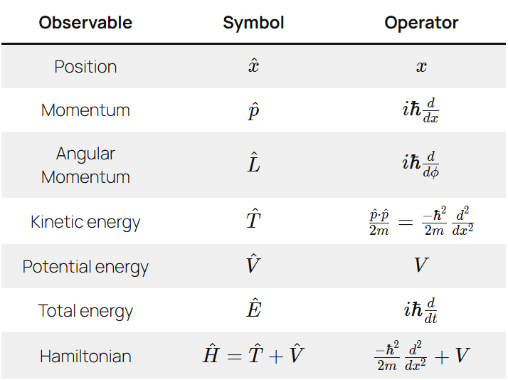
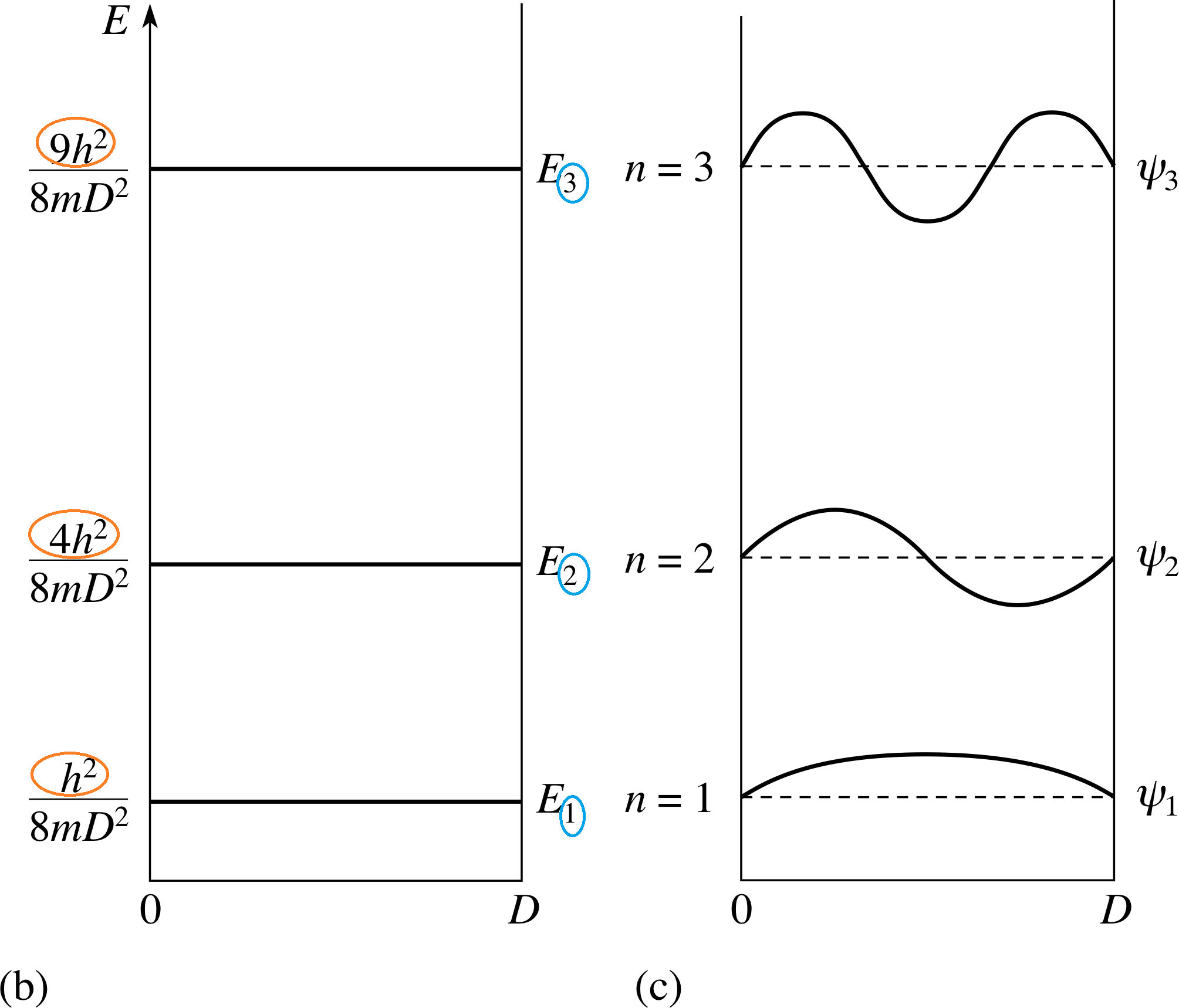
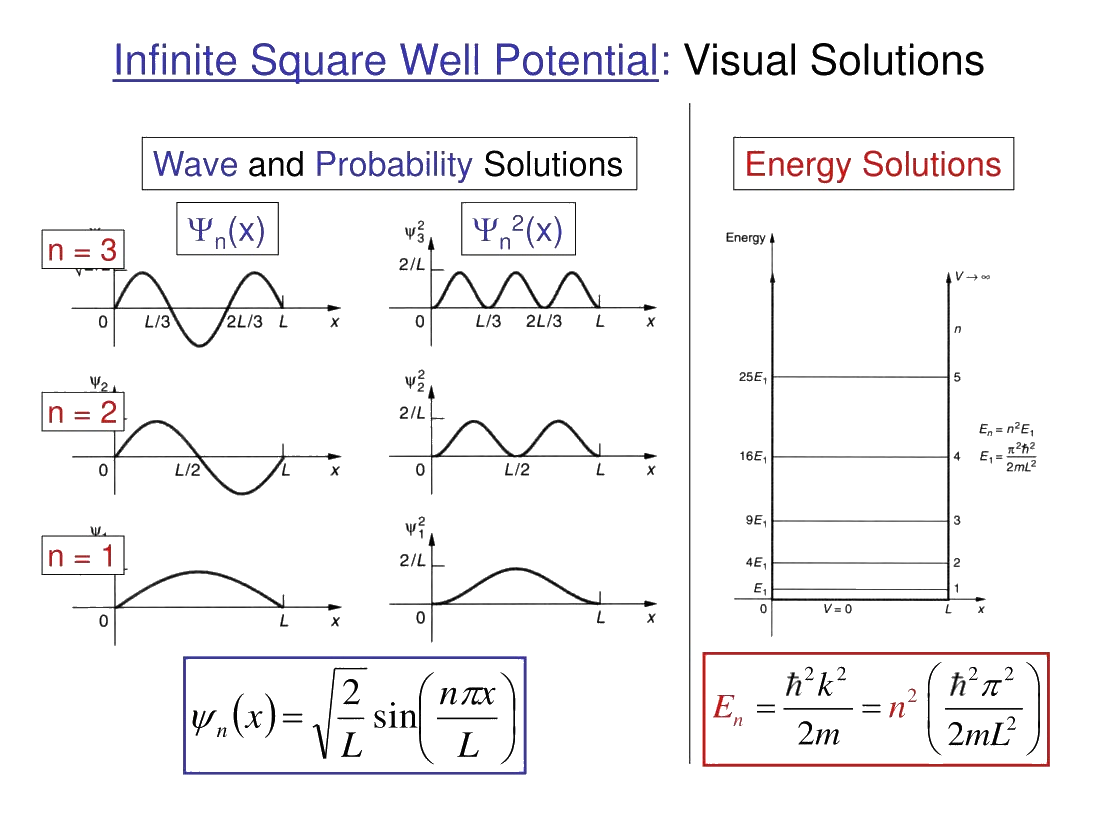
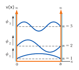
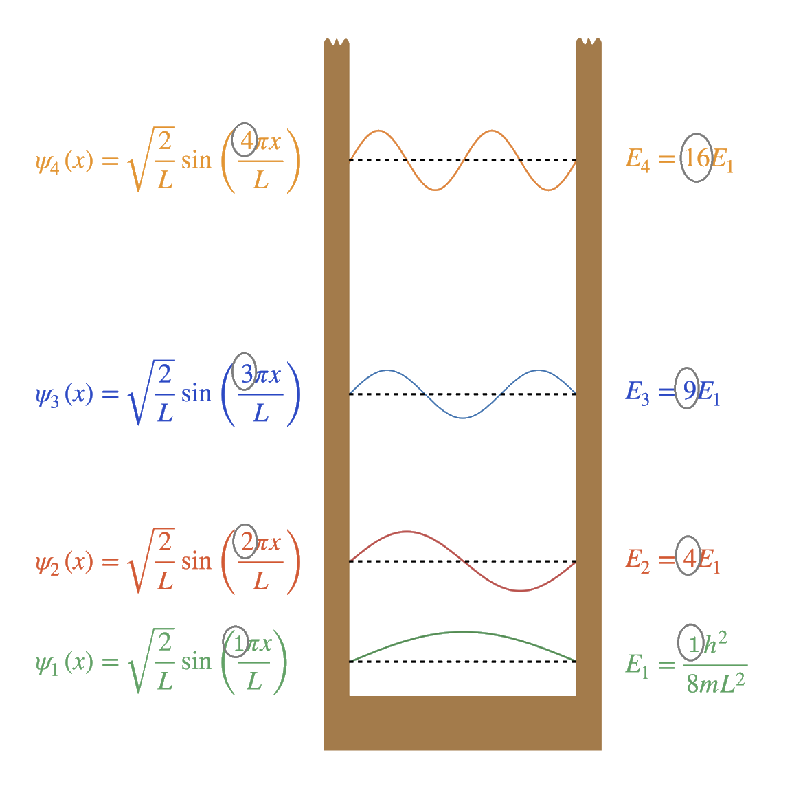
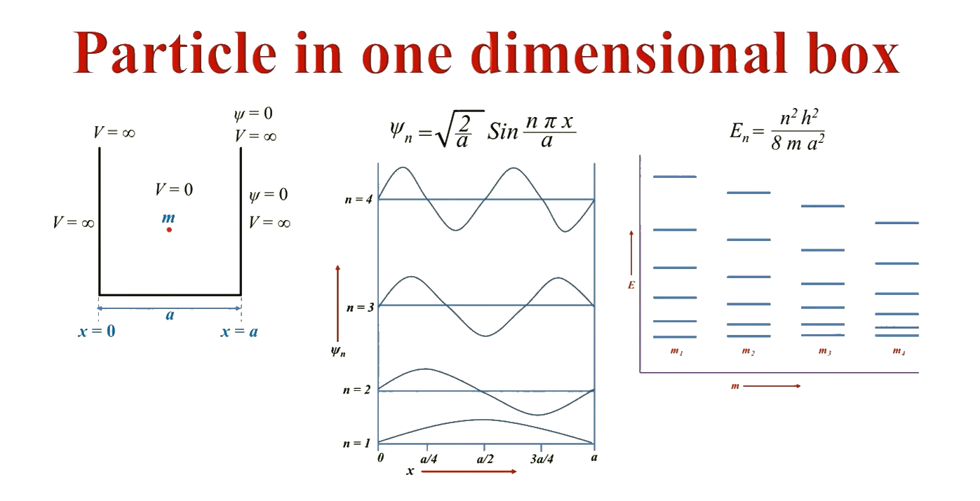
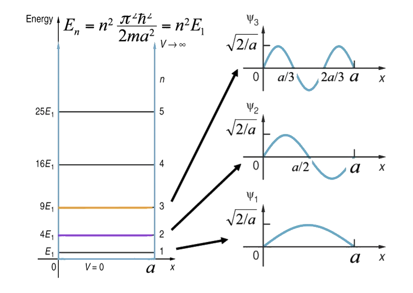
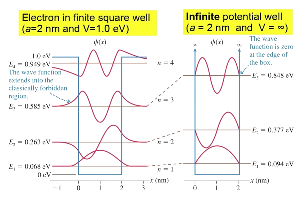
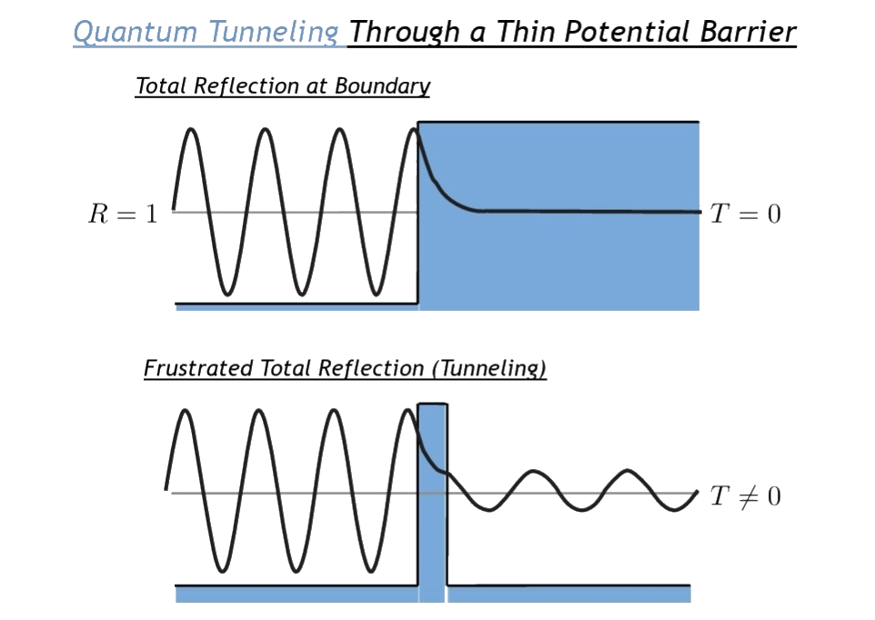
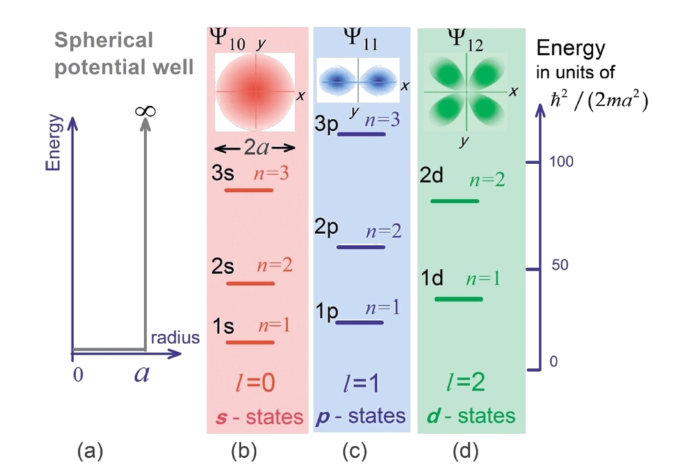
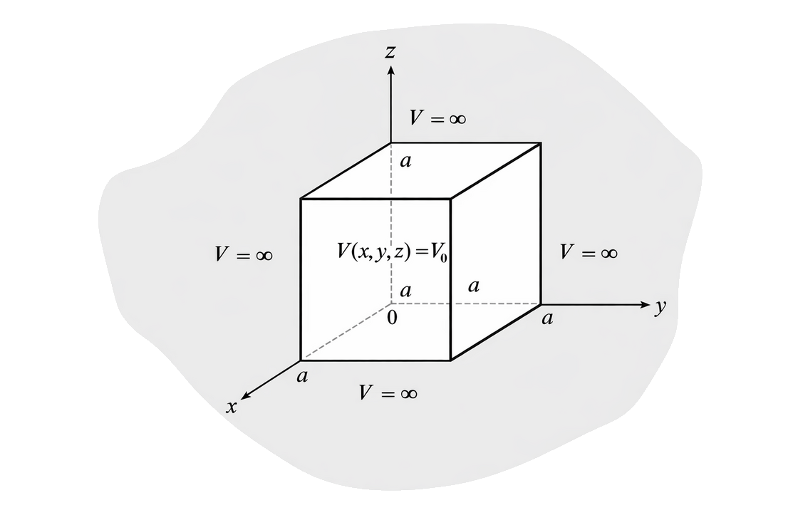
\(\hat H\psi_n=E_n\psi_n,\;\left\{\begin{array}{l}\psi_n(x)=\sqrt{\frac2a}\sin(\frac{n\pi x}a)\\E_n=\frac{n^2\pi^2\hslash^2}{2ma^2}\end{array}\right.,\;n=1,2,3,\cdots\)

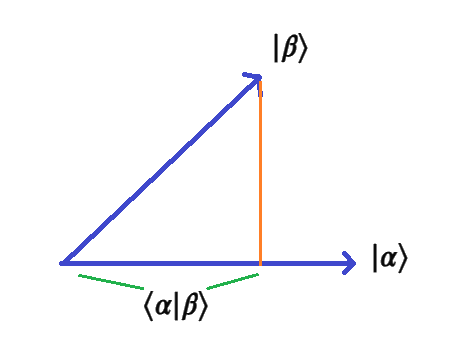
\(\int_0^a\psi_m^\ast(x)\psi_n(x)dx=\delta_{mn}\)

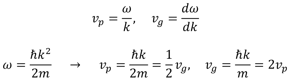
\(\psi(x)=\sum_nc_n\psi_n(x)\)

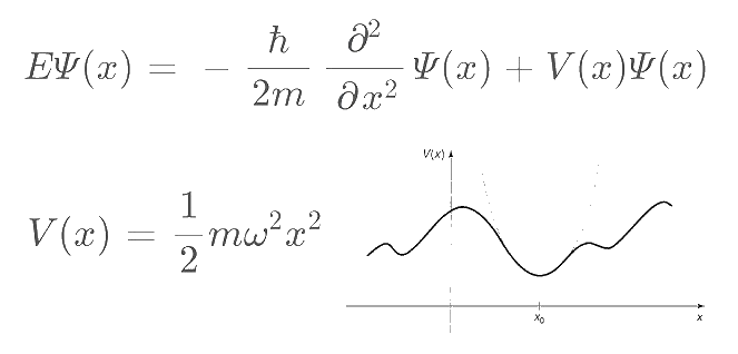
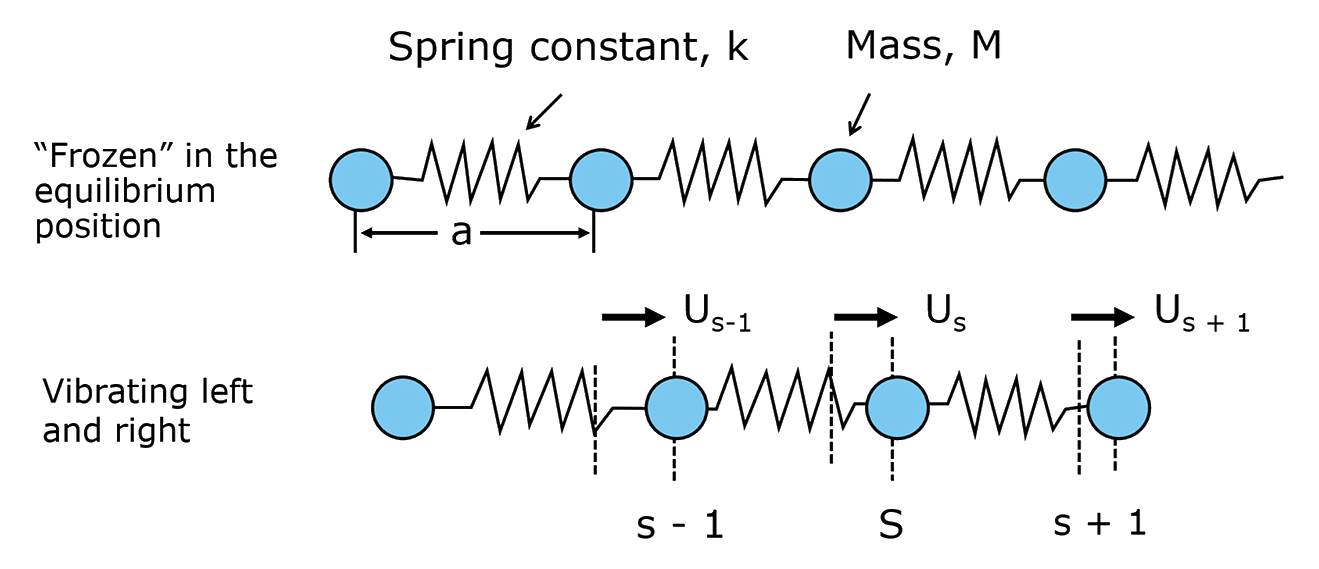
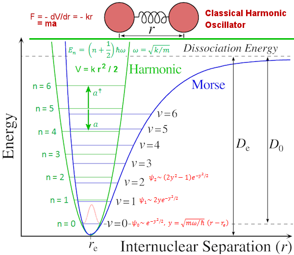
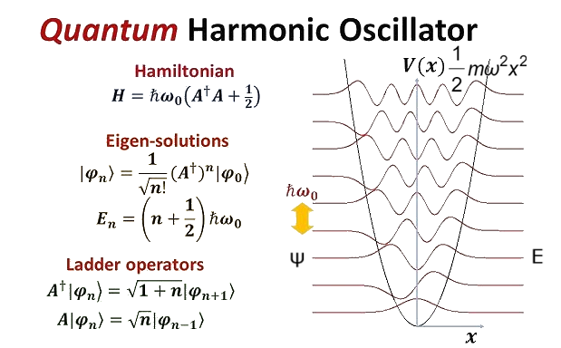
\(V(x)=\frac12m\omega^2x^2\)

Hooke's law - Spring potential energy
\(V(x)=\frac12kx^2\)

\(\omega=\sqrt{\frac km}\)

\(-\frac{\hslash^2}{2m}\frac{d^2\psi_n}{dx^2}+\frac12m\omega^2x^2\psi_n=E_n\psi_n\)

General, Common

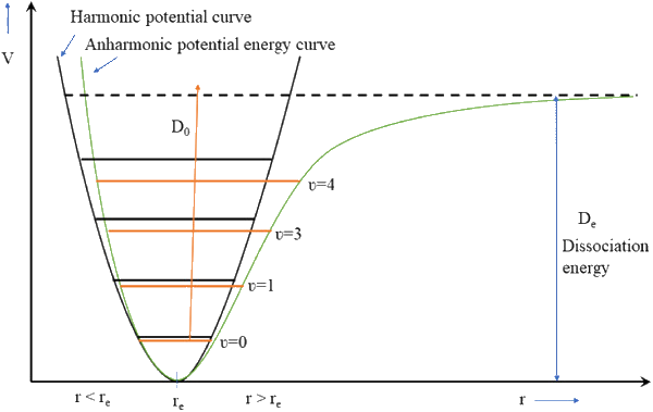
\(V(x)=\underbrace{V(x_0)}_{\equiv0}=\underbrace{V'(x_0)}_{=0}(x-x_0)+\frac12V''(x_0){(x-x_0)}^2+\underbrace\cdots_{anharmonic\;term\;(effect)}\)

\(x_0\simeq x\), near equilibrium

\(\frac{p^2}{2m}+\frac12m\omega^2x^2\psi=E\psi\)

\(\left\{\begin{array}{l}a_+\equiv\frac1{\sqrt{2m\hslash\omega}}(-ip+m\omega x)\\a_-\equiv\frac1{\sqrt{2m\hslash\omega}}(+ip+m\omega x)\end{array}\right.\)

\(a_-a_+=\frac1{2m\hslash\omega}(+ip+m\omega x)(-ip+m\omega x)\)
\(=\frac1{2m\hslash\omega}(p^2+m^2\omega^2x^2+im\omega px-im\omega xp)\)

\(\lbrack x,p\rbrack=xp-px\) "commutator"

\(\lbrack x,x\rbrack=x^2-x^2=0\)

\(\lbrack x,p\rbrack f(x)=xpf(x)-pxf(x)\)
\(=x\cdot\fracℏi\frac d{dx}f(x)-\fracℏi\frac d{dx}(xf(x))\)
\(=\cancel{x\cdot\fracℏi\frac{df(x)}{dx}}-\fracℏif(x)-\cancel{\fracℏi\cdot x\cdot\frac{df(x)}{dx}}\)
\(=i\hslash f(x)\)

\(\lbrack x,p\rbrack=i\hslash\)

\(a_-a_+=\frac1{2m\hslash\omega}(p^2+m^2\omega^2x^2+im\omega px-im\omega xp)\)
\(=\frac1{2m\hslash\omega}(p^2+m^2\omega^2x^2-im\omega\lbrack x,p\rbrack)\)
\(=\frac1{2m\hslash\omega}(p^2+m^2\omega^2x^2+m\hslash\omega)\)

\(\frac{p^2}{2m}+\frac12m\omega^2x^2\psi=E\psi\)

\(\underbrace{\frac1{2m}(p^2+m^2\omega^2x^2)}_\hat H\psi=E\psi\)

\(a_-a_+=\frac1{2m\hslash\omega}(p^2+m^2\omega^2x^2+m\hslash\omega)\)
\(=\frac1{2m\hslash\omega}(p^2+m^2\omega^2x^2)+\frac{1\cdot\cancel{m\hslash\omega}}{2\cdot\cancel{m\hslash\omega}}\)
\(=\frac1{\hslash\omega}\hat H+\frac12,\;\because\underbrace{\frac1{2m}(p^2+m^2\omega^2x^2)}_\hat H\psi=E\psi\)

\(\Rightarrow a_-a_+=\frac1{\hslash\omega}\hat H+\frac12\)
\(\Rightarrow \hat H=\hslash\omega(a_-a_+-\frac12)\)

\(a_-a_+=\frac1{2m\hslash\omega}(+ip+m\omega x)(-ip+m\omega x)\)
\(=\frac1{2m\hslash\omega}(p^2+m^2\omega^2x^2+im\omega px-im\omega xp)\)
\(=\frac1{2m\hslash\omega}(p^2+m^2\omega^2x^2-im\omega\lbrack x,p\rbrack)\)
\(=\frac1{2m\hslash\omega}(p^2+m^2\omega^2x^2+m\hslash\omega)\)
\(=\frac1{2m\hslash\omega}(p^2+m^2\omega^2x^2)+\frac{1\cdot\cancel{m\hslash\omega}}{2\cdot\cancel{m\hslash\omega}}\)
\(=\frac1{\hslash\omega}\hat H+\frac12,\;\because\frac1{2m}(p^2+m^2\omega^2x^2)=\hat H\)

\(\because a_-a_+=\frac1{\hslash\omega}\hat H+\frac12\)
\(\Rightarrow \hat H=\hslash\omega(a_-a_+-\frac12)\)

In quantum mechanics, the commutator of the position operator (x) and the momentum operator (p) is a fundamental concept. It represents the non-commutativity of these two operators, meaning the order in which they are applied to a wave function matters. The commutator [x, p] is defined as xp - px, and its value is equal to iħ (where i is the imaginary unit and ħ is the reduced Planck constant).

similarity

\(a_+a_-=\frac1{2m\hslash\omega}(-ip+m\omega x)(+ip+m\omega x)\)
\(=\frac1{2m\hslash\omega}(p^2+m^2\omega^2x^2-im\omega px+im\omega xp)\)
\(=\frac1{2m\hslash\omega}(p^2+m^2\omega^2x^2+im\omega\lbrack x,p\rbrack)\)
\(=\frac1{2m\hslash\omega}(p^2+m^2\omega^2x^2-m\hslash\omega)\)
\(=\frac1{2m\hslash\omega}(p^2+m^2\omega^2x^2)-\frac{1\cdot\cancel{m\hslash\omega}}{2\cdot\cancel{m\hslash\omega}}\)
\(=\frac1{\hslash\omega}\hat H-\frac12\)

\(\because a_+a_-=\frac1{\hslash\omega}\hat H-\frac12\)
\(\Rightarrow \hat H=\hslash\omega(a_+a_-+\frac12)\)

\(\left\{\begin{array}{l}\hslash\omega(a_-a_+-\frac12)\psi=E\psi\\\hslash\omega(a_+a_-+\frac12)\psi=E\psi\end{array}\right.\)

\(\lbrack a_-,a_+\rbrack=a_-a_+-a_+a_-=1\)

\(\left\{\begin{array}{l}\lbrack x,p\rbrack=i\hslash\\\lbrack a_-,a_+\rbrack=1\end{array}\right.\)

\(\left\{\begin{array}{l}\lbrack x^2,p\rbrack=?\\\lbrack x,p^2\rbrack=?\\\lbrack x^2,p^2\rbrack=?\end{array}\right.\)

(1) \(\lbrack x^2,p\rbrack=x\lbrack x,p\rbrack+\lbrack x,p\rbrack x\)
\(=xi\hslash+i\hslash x\)
\(=2i\hslash x\)

\(\therefore\lbrack x^n,p\rbrack=n\cdot i\hslash x^{n-1}\)

(2) \(\lbrack x,p^2\rbrack=\lbrack x,p\rbrack p+p\lbrack x,p\rbrack\)
\(=i\hslash p+pi\hslash\)
\(=2i\hslash p\)

\(\therefore\lbrack x,p^n\rbrack=n\cdot i\hslash p^{n-1}\)

(3) Using commutator identities,
To get past where you got, all you really have to do is use \(\lbrack x,p\rbrack=i\hslash\) once.

\(\lbrack x^2,p^2\rbrack=x\lbrack x,p^2\rbrack+\lbrack x,p^2\rbrack x\)
\(=x(\lbrack x,p\rbrack p+p\lbrack x,p\rbrack)+(\lbrack x,p\rbrack p+p\lbrack x,p\rbrack)x\)
\(=x\lbrack x,p\rbrack p+xp\lbrack x,p\rbrack+\lbrack x,p\rbrack px+p\lbrack x,p\rbrack x\)
\(=xi\hslash p+xpi\hslash+i\hslash px+pi\hslash x\)
\(=2i\hslash(xp+px)\)
\(=2i\hslash(xp+(xp-i\hslash))\)
\(=4i\hslash xp+2\hslash^2\)

\(\lbrack x,p\rbrack=xp-px=i\hslash\)
\(-(xp-px)=-i\hslash\)
\(px-xp=-i\hslash=\lbrack p,x\rbrack\)
\(px=xp-i\hslash\)

---

\(\left\{\begin{array}{l}\lbrack A,B\rbrack=AB-BA\\\lbrack A,BC\rbrack=\lbrack A,B\rbrack C+B\lbrack A,C\rbrack\\\lbrack AB,C\rbrack=A\lbrack B,C\rbrack+\lbrack A,C\rbrack B\end{array}\right.\)

\([AB,C] = (AB)C - C(AB) = ABC - CAB\)

Now, let's look at the right-hand side. The RHS has two terms: \(A[B,C]\) and \([A,C]B\)

\(A[B,C] = A(BC - CB) = ABC - ACB\)
\([A,C]B = (AC-CA)B = ACB - CAB\)

So in fact, the correct formula looks like:

\(\begin{align} A[B,C]+[A,C]B&= ABC - ACB + ACB - CAB\\ & = ABC - CAB \\ & = [AB,C] \end{align}\)

So, \([AB,C] = A[B,C]+[A,C]B\)

\([A,BC]=A(BC)-(BC)A=ABC-BCA\)

Now, let's look at the right-hand side. The RHS has two terms: \(B[A,C]\) and \([A,B]C\)

\(B[A,C]=B(AC-CA)=BAC-BCA\)
\([A,B]C=(AB-BA)C=ABC-BAC\)

So in fact, the correct formula looks like:

\(\begin{align} B[A,C]+[A,B]C&=BAC-BCA+ABC-BAC\\ & =ABC-BCA \\ & = [A,BC] \end{align}\)

So, \([A,BC] = B[A,C]+[A,B]C\)

\(\left\{\begin{array}{l}\lbrack x,p\rbrack=i\hslash\\\lbrack x^2,p\rbrack=\lbrack x\cdot x,p\rbrack=x\lbrack x,p\rbrack+\lbrack x,p\rbrack x=i\hslash x+i\hslash x=2i\hslash x\\\lbrack x^3,p\rbrack=\lbrack x\cdot x^2,p\rbrack=x\lbrack x^2,p\rbrack+\lbrack x,p\rbrack x^2=2i\hslash x\cdot x+i\hslash x^2=3i\hslash x^2\\\lbrack x^4,p\rbrack=\lbrack x\cdot x^3,p\rbrack=x\lbrack x^3,p\rbrack+\lbrack x,p\rbrack x^3=3i\hslash x^2\cdot x+i\hslash x^3=4i\hslash x^3\end{array}\right.\)

\(\therefore\lbrack x^n,p\rbrack=\lbrack x\cdot x^{n-1},p\rbrack=ni\hslash x^{n-1}\)

\(\left\{\begin{array}{l}\lbrack x,p\rbrack=i\hslash\\\lbrack x,p^2\rbrack=\lbrack x,p\cdot p\rbrack=p\lbrack x,p\rbrack+\lbrack x,p\rbrack p=i\hslash p+i\hslash p=2i\hslash p\\\lbrack x,p^3\rbrack=\lbrack x,p^2\cdot p\rbrack=p^2\lbrack x,p\rbrack+\lbrack x,p^2\rbrack p=i\hslash p^2+2i\hslash p\cdot p=3i\hslash p^2\\\lbrack x,p^4\rbrack=\lbrack x,p^3\cdot p\rbrack=p^3\lbrack x,p\rbrack+\lbrack x,p^3\rbrack p=i\hslash p^3+3i\hslash p^2\cdot p=4i\hslash p^3\end{array}\right.\)

\(\therefore\lbrack x,p^n\rbrack=\lbrack x,p^{n-1}p\rbrack=ni\hslash p^{n-1}\)

Generalizations

\(\lbrack F(\vec x),p_i\rbrack=i\hslash\frac{\partial F(\vec x)}{\partial x_i};\qquad\lbrack x_i,F(\vec p)\rbrack=i\hslash\frac{\partial F(\vec p)}{\partial p_i}.\)

using \(C_{n+1}^{k}=C_{n}^{k}+C_{n}^{k-1}\), it can be shown that by mathematical induction

\(\left[\widehat x^n,\widehat p^m\right]=\sum_{k=1}^{\min\left(m,n\right)}\frac{-\left(-i\hslash\right)^kn!m!}{k!\left(n-k\right)!\left(m-k\right)!}\widehat x^{n-k}\widehat p^{m-k}=\sum_{k=1}^{\min\left(m,n\right)}\frac{\left(i\hslash\right)^kn!m!}{k!\left(n-k\right)!\left(m-k\right)!}\widehat p^{m-k}\widehat x^{n-k}\)

generally known as McCoy's formula.

\(-\frac{\hslash^2}{2m}\frac{d^2\psi}{dx^2}+\frac12m\omega^2x^2\psi=E\psi\)
\(a_\pm\equiv\frac1{\sqrt{2m\hslash\omega}}(\mp ip+m\omega x)\)
\(\lbrack x,p\rbrack=i\hslash\)
\(\lbrack a_-,a_+\rbrack=1\)
\(\lbrack A,B\rbrack=AB-BA\)

\(H\psi_n=E_n\psi_n\)
\(H=\hslash\omega(a_+a_-+\frac12)\)
\(H=\hslash\omega(a_-a_+-\frac12)\)

if \(\psi\) is a solution with eigenvalue \(E\), \(H\psi=E\psi\)
then \(a_+\psi\) is a solution too, with eigenvalue \(E+\hslash\omega\)

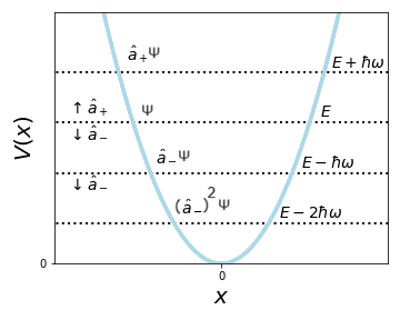
Proof: \(H(a_+\psi)\)
\(=(\hslash\omega(a_+a_-+\frac12))(a_+\psi)\)
\(=\hslash\omega(a_+a_-)(a_+\psi)+\frac12\hslash\omega(a_+\psi)\)
\(=\hslash\omega(a_+a_-a_+\psi)+\frac12\hslash\omega(a_+\psi)\)
\(=a_+(\hslash\omega(a_-a_+\psi+\frac12\psi))\)
\(\because\lbrack a_-,a_+\rbrack=1\;\Rightarrow\;a_-a_+-a_+a_-=1\;\Rightarrow\;a_-a_+=a_+a_-+1\)
\(=a_+(\hslash\omega((a_+a_-+1)\psi+\frac12\psi))\)
\(=a_+(\underbrace{\hslash\omega((a_+a_-+\frac12)}_H\psi+1\cdot\psi))\)
\(=a_+(H\psi+\hslash\omega\psi)\)
\(=a_+(E\psi+\hslash\omega\psi)\)
\(=(E+\hslash\omega)(a_+\psi)\)

\(H(a_-\psi)\)
\(=(\hslash\omega(a_-a_+-\frac12))(a_-\psi)\)
\(=\hslash\omega(a_-a_+)(a_-\psi)-\frac12\hslash\omega(a_-\psi)\)
\(=\hslash\omega(a_-a_+a_-\psi)-\frac12\hslash\omega(a_-\psi)\)
\(=a_-(\hslash\omega(a_+a_-\psi-\frac12\psi))\)
\(\because\lbrack a_+,a_-\rbrack=-1\;\Rightarrow\;a_+a_--a_-a_+=-1\;\Rightarrow\;a_+a_-=a_-a_+-1\)
\(=a_-(\hslash\omega((a_-a_+-1)\psi-\frac12\psi))\)
\(=a_-(\underbrace{\hslash\omega((a_-a_+-\frac12)}_H\psi-1\cdot\psi))\)
\(=a_-(H\psi-\hslash\omega\psi)\)
\(=a_-(E\psi-\hslash\omega\psi)\)
\(=(E-\hslash\omega)(a_-\psi)\)

\(\left\{\begin{array}{l}H(a_+\psi)=(E+\hslash\omega)(a_+\psi)\\H(a_-\psi)=(E-\hslash\omega)(a_-\psi)\end{array}\right.\)

\(\left\{\begin{array}{l}H(a_+\psi)=(E+\hslash\omega)(a_+\psi)\\H(a_+^2\psi)=(E+2\hslash\omega)(a_+\psi)\\H(a_+^3\psi)=(E+3\hslash\omega)(a_+\psi)\end{array}\right.\)

\(\left\{\begin{array}{l}H(a_-\psi)=(E-\hslash\omega)(a_-\psi)\\H(a_-^2\psi)=(E-2\hslash\omega)(a_-\psi)\\H(a_-^3\psi)=(E-3\hslash\omega)(a_-\psi)\end{array}\right.\)

if \(\psi\) is a solution with eigenvalue \(E\), \(H\psi=E\psi\)
then \(a_+\psi\) is a solution too, with eigenvalue \(E+\hslash\omega\)
then \(a_-\psi\) is a solution too, with eigenvalue \(E-\hslash\omega\)

\(E_n＞0\)

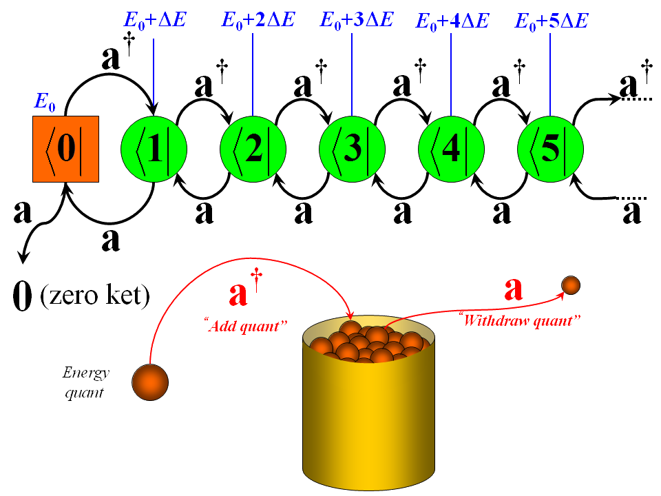
\(a_+\): raising operator
\(a_-\): lowering operator

\(a_\pm\equiv\frac1{\sqrt{2m\hslash\omega}}(\mp ip+m\omega x)\)

\(H\psi_0=E_0\psi_0\)

\(a_-\psi_0=0\)

\(a_-=\frac1{\sqrt{2m\hslash\omega}}(+ip+m\omega x)\)

\((i\fracℏi\frac d{dx}+m\omega x)\psi_0(x)=0\)

\(\frac{d\psi_0}{dx}=-\frac{m\omega}ℏx\psi_0\)

\(\frac{d\psi_0}{\psi_0}=-\frac{m\omega}ℏxdx\)

\(\ln(\psi_0)=-\frac{m\omega x^2}{2\hslash}+c\)

\(\Rightarrow\psi_0(x)=Ae^{-\frac{m\omega}{2\hslash}x^2}\)

\(\because\int_{-\infty}^\infty\left|\psi_0(x)\right|^2\operatorname dx=1\)
\(\Rightarrow A={(\frac{m\omega}{\pi\hslash})}^\frac14\)
\(\Rightarrow\psi_0(x)={(\frac{m\omega}{\pi\hslash})}^\frac14e^{-\frac{m\omega}{2\hslash}x^2}\)

\(\hslash\omega(a_+a_-+\frac12)\psi_0=E_0\psi_0\)
\(\because a_-\psi_0=0\;\Rightarrow\;a_+a_-\psi_0=0\;\Rightarrow\;\hslash\omega(a_+a_-)\psi_0=0\)
\(\frac12\hslash\omega\psi_0=E_0\psi_0\)

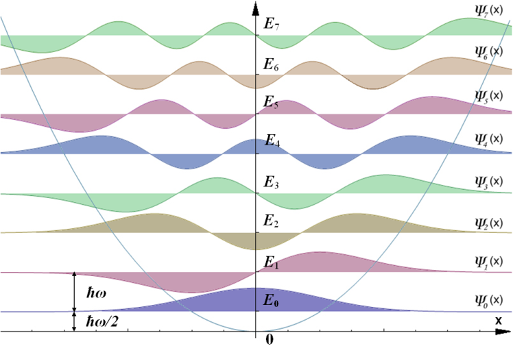
\(\therefore\psi_0\;\rightarrow\;E_0=\frac12\hslash\omega\)

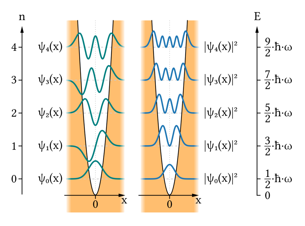
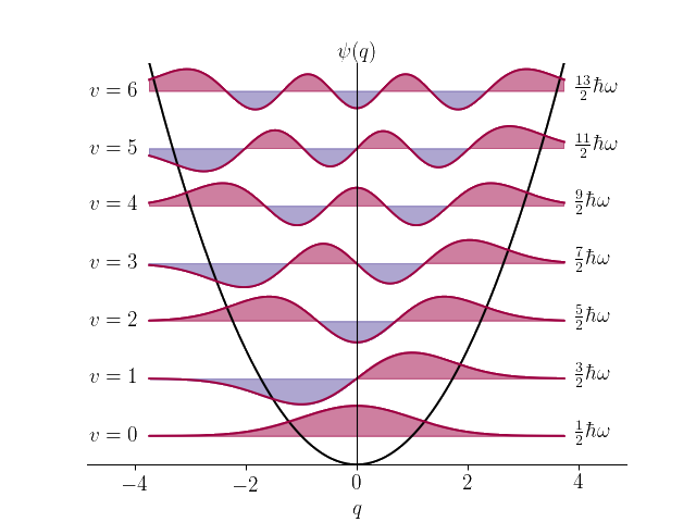
\(\left\{\begin{array}{l}\psi_n=A_n{(a_+)}^n\psi_0\;(x)\\E_n=(n+\frac12)\hslash\omega\end{array}\right.\)

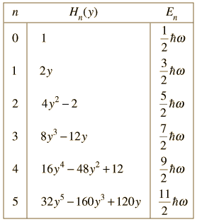
\(\psi_1\propto x\cdot e^{-\frac{m\omega}{2\hslash}x^2}\)

\(\psi_2\propto x^2\cdot e^{-\frac{m\omega}{2\hslash}x^2}\)

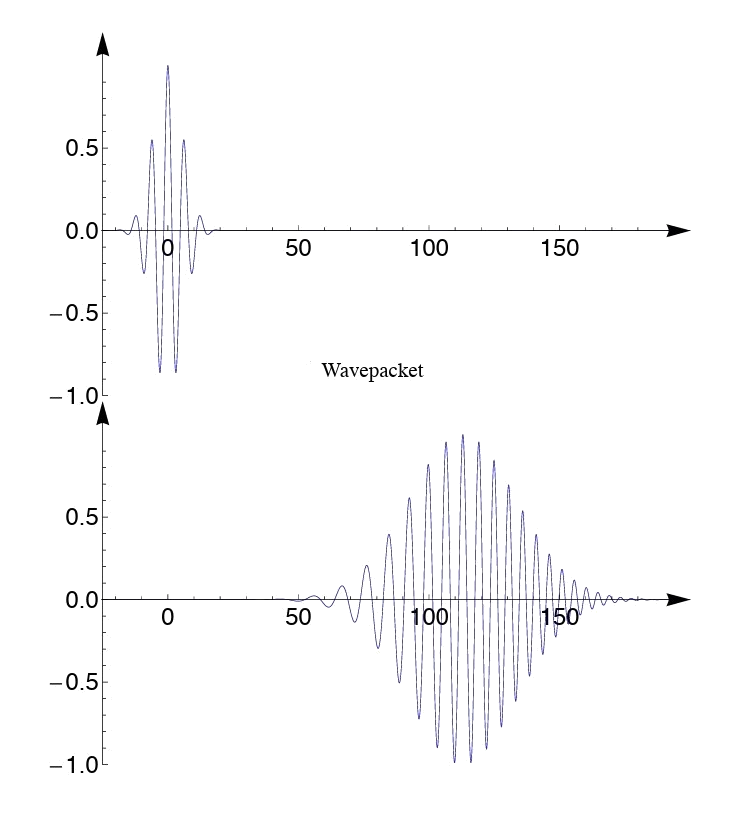
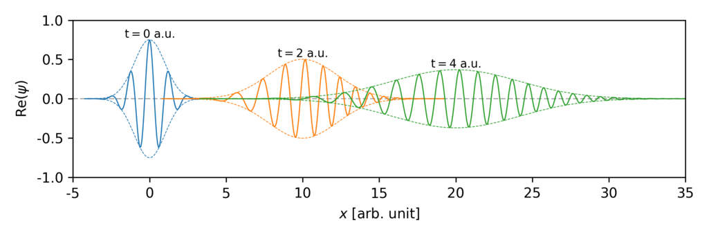
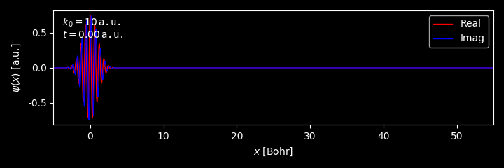
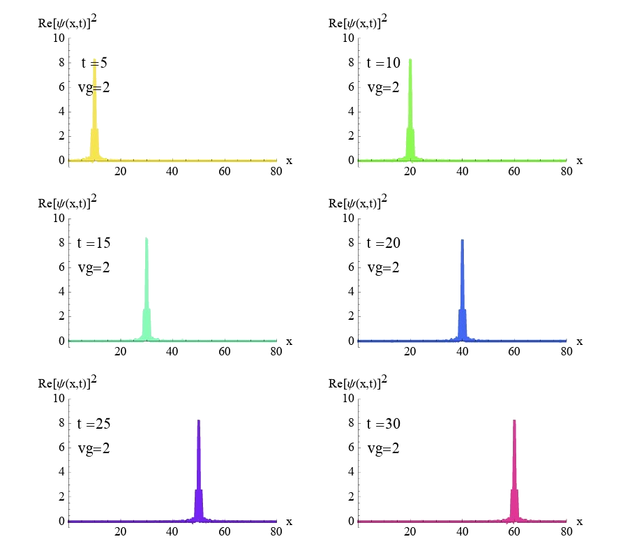
\(\Psi(x,t)=\sum_nc_n\psi_ne^{-\frac{iE_n}ℏt}\)

\(\left\langle\hat Q(x,p)\right\rangle=\int\Psi^\ast Q\Psi dx\)

\(\left\{\begin{array}{l}a_+\psi_n=c_n\psi_{n+1}\\a_-\psi_n=d_n\psi_{n-1}\end{array}\right.\)

\(\int_{-\infty}^{+\infty}f^\ast(x)(a_+g(x))\operatorname dx\)
\(=\int_{-\infty}^{+\infty}f^\ast(-i\fracℏi\frac d{dx}+m\omega x)g\operatorname dx\)

\(\int_{-\infty}^{+\infty}f^\ast(-\hslash\frac{dg}{dx})dx=-\hslash(\cancel{\left.f^\ast g\right|_{-\infty}^\infty}-\int\frac{df^\ast}{dx}gdx)\)
\(=\hslash\int\frac{df^\ast}{dx}gdx\)

\(\Rightarrow\int_{-\infty}^{+\infty}f^\ast(-i\fracℏi\frac d{dx}+m\omega x)g\operatorname dx\)
\(=\int_{-\infty}^{+\infty}({(i\fracℏi\frac d{dx}+m\omega x)f)}^\ast gdx\)
\(=\int_{-\infty}^{+\infty}{(a_-f)}^\ast gdx\)

\(\int_{-\infty}^{+\infty}f^\ast(x)(a_+g(x))\operatorname dx=\int_{-\infty}^{+\infty}{(a_-f(x))}^\ast g(x)dx\)

\(H=\hslash\omega(a_+a_-+\frac12)=\hslash\omega(a_-a_+-\frac12)\)
\(H\psi_n=E_n\psi_n\)

\(\hslash\omega(a_+a_-+\frac12)\psi_n=E_n\psi_n=(n+\frac12)\hslash\omega\psi_n\)
\(\hslash\omega(a_+a_-+\cancel{\frac12})\psi_n=(n+\cancel{\frac12})\hslash\omega\psi_n\)

\(\hslash\omega(a_-a_+-\frac12)\psi_n=E_n\psi_n=(n+\frac12)\hslash\omega\psi_n=\lbrack(n+1)-\frac12\rbrack\hslash\omega\psi_n\)
\(\hslash\omega(a_-a_+-\cancel{\frac12})\psi_n=\lbrack(n+1)-\cancel{\frac12}\rbrack\hslash\omega\psi_n\)

number operator \(\left\{\begin{array}{l}a_+a_-\psi_n=n\psi_n\\a_-a_+\psi_n=(n+1)\psi_n\end{array}\right.\)

\(\left\{\begin{array}{l}a_+\psi_n=c_n\psi_{n+1}\\a_-\psi_n=d_n\psi_{n-1}\end{array}\right.\)

number operator \(\left\{\begin{array}{l}a_+a_-\psi_n=n\psi_n\\a_-a_+\psi_n=(n+1)\psi_n\end{array}\right.\)

\(\because a_+\psi_n=c_n\psi_{n+1}\)
\(\int_{-\infty}^\infty{(a_+\psi_n)}^\ast(a_+\psi_n)\operatorname dx=\int_{-\infty}^\infty{(c_n\psi_{n+1})}^\ast(c_n\psi_{n+1})\operatorname dx\)
\(=\int_{-\infty}^\infty{(a_-a_+\psi_n)}^\ast\psi_n\operatorname dx\)
\(=\int_{-\infty}^\infty{(n+1)\psi_n}^\ast\psi_n\operatorname dx\)
\(=n+1\)

\(\int_{-\infty}^\infty{(c_n\psi_{n+1})}^\ast(c_n\psi_{n+1})\operatorname dx=\left|c_n\right|^2\underbrace{\int_{-\infty}^\infty\left|\psi_{n+1}\right|^2dx}_{=1}\)
\(=\left|c_n\right|^2\)

\(\therefore c_n=\sqrt{n+1}\)

\(\because a_-\psi_n=d_n\psi_{n-1}\)
\(\int_{-\infty}^\infty{(a_-\psi_n)}^\ast(a_-\psi_n)\operatorname dx=\int_{-\infty}^\infty{(d_n\psi_{n-1})}^\ast(d_n\psi_{n-1})\operatorname dx\)
\(=\int_{-\infty}^\infty{(a_+a_-\psi_n)}^\ast\psi_n\operatorname dx\)
\(=\int_{-\infty}^\infty{n\cdot\psi_n}^\ast\psi_n\operatorname dx\)
\(=n\)

\(\int_{-\infty}^\infty{(d_n\psi_{n-1})}^\ast(d_n\psi_{n-1})\operatorname dx=\left|d_n\right|^2\underbrace{\int_{-\infty}^\infty\left|\psi_{n-1}\right|^2dx}_{=1}\)
\(=\left|d_n\right|^2\)

\(\therefore d_n=\sqrt n\)

\(\left\{\begin{array}{l}c_n=\sqrt{n+1}\\d_n=\sqrt n\end{array}\right.\)

\(\Rightarrow\left\{\begin{array}{l}a_+\psi_n=\sqrt{n+1}\psi_{n+1}\\a_-\psi_n=\sqrt n\psi_{n-1}\end{array}\right.\)

---

\(a_+\psi_n=\sqrt{n+1}\psi_{n+1}\;\Rightarrow\psi_{n+1}=\frac{a_+}{\sqrt{n+1}}\psi_n\)
\(\psi_1=a_+\psi_0\)
\(\psi_2=\frac1{\sqrt2}a_+\psi_1=\frac1{\sqrt2}{(a_+)}^2\psi_0\)
\(\psi_3=\frac1{\sqrt3}a_+\psi_2=\frac1{\sqrt3}\frac1{\sqrt2}{(a_+)}^2\psi_1=\frac1{\sqrt3}\frac1{\sqrt2}\frac1{\sqrt1}{(a_+)}^3\psi_0\)

\(\psi_n(x)=\frac1{\sqrt{n!}}{(a_+)}^n\psi_0(x)\)

\(\Rightarrow\left\{\begin{array}{l}\psi_n(x)=\frac1{\sqrt{n!}}{(a_+)}^n\psi_0(x)\;\Rightarrow\vert n\rangle=\frac1{\sqrt{n!}}{(a_+)}^n\vert0\rangle\\E_n=(n+\frac12)\hslash\omega\end{array}\right.\)

\(\langle\hat Q(x,p)\rangle=?\)

\(\langle x\rangle=\langle n\vert x\vert n\rangle=\int_{-\infty}^\infty\psi_n^\ast(x)\cdot x\cdot\psi_n(x)\operatorname dx=?\)

number operator \(\left\{\begin{array}{l}a_+a_-\psi_n=n\psi_n\\a_-a_+\psi_n=(n+1)\psi_n\end{array}\right.\)

\(\int_{-\infty}^\infty\psi_m^\ast\psi_n\operatorname dx,\;m\neq n\)
\(=\frac1n\int_{-\infty}^\infty\psi_m^\ast n\psi_n\operatorname dx\)
\(=\frac1n\int_{-\infty}^\infty\psi_m^\ast(a_+a_-\psi_n)\operatorname dx\)
\(=\frac1n\int_{-\infty}^\infty\psi_m^\ast a_+(a_-\psi_n)\operatorname dx\)
\(=\frac1n\int_{-\infty}^\infty\underbrace{\psi_m^\ast a_+}(a_-\psi_n)\operatorname dx\)
\(=\frac1n\int_{-\infty}^\infty\underbrace{{(a_-\psi_m)}^\ast(a_-}\psi_n)\operatorname dx\)
\(=\frac1n\int_{-\infty}^\infty{(a_+a_-\psi_m)}^\ast(\psi_n)\operatorname dx\)
\(=\frac1n\int_{-\infty}^\infty{m\psi_m}^\ast\psi_n\operatorname dx\)

\(\Rightarrow\int_{-\infty}^\infty\psi_n^\ast\psi_n\operatorname dx=\frac mn\int_{-\infty}^\infty\psi_m^\ast\psi_n\operatorname dx\)
\((m-n)\int_{-\infty}^\infty\psi_m^\ast\psi_n\operatorname dx=0\)
\(\therefore\int_{-\infty}^\infty\psi_m^\ast\psi_n\operatorname dx=0\)

\(\langle x\rangle=?\)

\(\left\{\begin{array}{l}a_+=\frac1{\sqrt{2m\hslash\omega}}(-ip+m\omega x)\;\;\cdots\;(\alpha)\\a_-=\frac1{\sqrt{2m\hslash\omega}}(+ip+m\omega x)\;\;\cdots\;(\beta)\end{array}\right.\)

\((\alpha)+(\beta)\;\Rightarrow\;x=\frac1{2m\omega}\sqrt{2m\hslash\omega}(a_++a_-)\)
\(\therefore x=\sqrt{\fracℏ{2m\omega}}(a_++a_-)\)

\((\beta)-(\alpha)\;\Rightarrow\;p=\frac1{2i}\sqrt{2m\hslash\omega}(a_--a_+)\)
\(\therefore p=i\sqrt{\frac{m\hslash\omega}2}(a_+-a_-)\)

\(\langle x\rangle=\int_{-\infty}^\infty\psi_n^\ast\cdot x\cdot\psi_n\operatorname dx,\;and\;applied\;x=\sqrt{\fracℏ{2m\omega}}(a_++a_-)\)
\(=\int_{-\infty}^\infty\psi_n^\ast(\sqrt{\fracℏ{2m\omega}}(a_++a_-))\psi_n\operatorname dx\)
\(=\sqrt{\fracℏ{2m\omega}}(\int_{-\infty}^\infty\psi_n^\ast a_+\psi_n\operatorname dx+\int_{-\infty}^\infty\psi_n^\ast a_-\psi_n\operatorname dx)\)
\(\Rightarrow\left\{\begin{array}{l}a_+\psi_n=\sqrt{n+1}\psi_{n+1}\\a_-\psi_n=\sqrt n\psi_{n-1}\end{array}\right.\)
\(=\sqrt{\fracℏ{2m\omega}}(\int_{-\infty}^\infty\psi_n^\ast\sqrt{n+1}\psi_{n+1}\operatorname dx+\int_{-\infty}^\infty\psi_n^\ast\sqrt n\psi_{n-1}\operatorname dx)\)
\(\langle x\rangle=0\) ◼

\(\langle x\rangle=0,\;\langle x^2\rangle=?\)

\(\because x=\sqrt{\fracℏ{2m\omega}}(a_++a_-)\)
\(x^2=\fracℏ{2m\omega}(a_++a_-)(a_++a_-)\)
\(=\fracℏ{2m\omega}(a_+^2+a_+a_-+a_-a_++a_-^2)\)
\(\langle x^2\rangle=\fracℏ{2m\omega}\int_{-\infty}^\infty\psi_n^\ast(a_+^2+a_+a_-+a_-a_++a_-^2)\psi_n\operatorname dx\)
\(=\fracℏ{2m\omega}\int_{-\infty}^\infty\psi_n^\ast(\underbrace{\cancel{a_+^2}}_{\psi_{n+2}}+a_+a_-+a_-a_++\underbrace{\cancel{a_-^2}}_{\psi_{n-2}})\psi_n\operatorname dx\)
\(=\fracℏ{2m\omega}\int_{-\infty}^\infty\psi_n^\ast(\underbrace{a_+a_-}_{\sqrt n\sqrt n}+\underbrace{a_-a_+}_{\sqrt{n+1}\sqrt{n+1}})\psi_n\operatorname dx\;\because\left\{\begin{array}{l}a_+\psi_n=\sqrt{n+1}\psi_{n+1}\\a_-\psi_n=\sqrt n\psi_{n-1}\end{array}\right.\)
\(=\fracℏ{2m\omega}(2n+1)\) ◼

\(\langle V\rangle=\langle\frac12m\omega^2x^2\rangle\)
\(=\frac12m\omega^2\langle x^2\rangle\)
\(=\frac12m\omega^2\cdot\fracℏ{2m\omega}(2n+1)\)
\(=\frac12\hslash\omega(n+\frac12)\)

\(\therefore\langle V\rangle=\frac12E_n\)

\(\langle K\rangle=\frac1{2m}\langle p^2\rangle\)

Bloch's theorem

In condensed matter physics, Bloch's theorem states that solutions to the Schrödinger equation in a periodic potential can be expressed as plane waves modulated by periodic functions.

Bloch function

\(\psi(\mathbf r)=e^{i\mathbf k\cdot\mathbf r}u(\mathbf r)\)

where \(\mathbf {r}\) is position, \(\psi\) is the wave function, \(u\) is a periodic function with the same periodicity as the crystal, the wave vector \(\mathbf {k}\) is the crystal momentum vector, \(e\) is Euler's number, and \(i\) is the imaginary unit.

Functions of this form are known as Bloch functions or Bloch states, and serve as a suitable basis for the wave functions or states of electrons in crystalline solids.

The description of electrons in terms of Bloch functions, termed Bloch electrons (or less often Bloch Waves), underlies the concept of electronic band structures.

These eigenstates are written with subscripts as \(\psi _{n\mathbf {k} }\), where \(n\) is a discrete index, called the band index

Solid line: A schematic of the real part of a typical Bloch state in one dimension. The dotted line is from the factor \(e^{i\mathbf k\cdot\mathbf r}\). The light circles represent atoms.

A Bloch wave function (bottom) can be broken up into the product of a periodic function (top) and a plane-wave (center). The left side and right side represent the same Bloch state broken up in two different ways, involving the wave vector \(k_1\) (left) or \(k_2\) (right). The difference (\(k_1−k_2\)) is a reciprocal lattice vector. In all plots, blue is real part and red is imaginary part.

Isosurface of the square modulus of a Bloch state in a silicon lattice

Quantum Operator

Observable Name	Symbol	Operator in QM	Operation
Position	\({\bf r}\)	\(\hat{\bf r}\)	Multiply by \({\bf r}\)
Momentum	\({\bf p}\)	\(\hat{\bf p}\)	\(-i \hbar \left(\hat{i}\dfrac{\partial}{\partial x} +\hat{j} \dfrac{\partial}{\partial y}+\hat{k} \dfrac{\partial}{\partial z} \right)\)
	\(p_x\)	\(\hat p_x\)	\(-i \hbar \dfrac{\partial}{\partial x}\)
	\(p_y\)	\(\hat p_y\)	\(-i \hbar \dfrac{\partial}{\partial y}\)
	\(p_z\)	\(\hat p_z\)	\(-i \hbar \dfrac{\partial}{\partial z}\)
Kinetic energy	\(T\)	\(\hat{T}\)	\(- \dfrac{\hbar^2}{2m} \left(\dfrac{\partial^2}{\partial x^2} +\dfrac{\partial^2}{\partial y^2} +\dfrac{\partial^2}{\partial z^2} \right)\)
Potential energy	\(V({\bf r})\)	\(\hat{V}({\bf r})\)	Multiply by \(V({\bf r})\)
Total energy	\(E\)	\(\hat{H}\)	\(-\dfrac{\hbar^2}{2m} \left(\dfrac{\partial^2}{\partial x^2} +\dfrac{\partial^2}{\partial y^2} +\dfrac{\partial^2}{\partial z^2} \right) +V({\bf r})\)
Angular momentum	\(L\)	\(\hat{L}^2\)	\(\hat{L}_x^2+\hat{L}_y^2+\hat{L}_z^2\)
	\(L_x\)	\(\hat{L}_x\)	\(-i\hbar\left(y\dfrac{\partial}{\partial z} - z \dfrac{\partial}{\partial y} \right)\)
	\(L_y\)	\(\hat{L}_y\)	\(-i \hbar \left(z\dfrac{\partial}{\partial x} - x \dfrac{\partial}{\partial z} \right)\)
	\(L_z\)	\(\hat{L}_z\)	\(-i \hbar \left(x\dfrac{\partial}{\partial y} - y \dfrac{\partial}{\partial x} \right)\)

Schrodinger: A prologue inferring the Wave Equation for Light

\(\psi\approx e^{j(\omega t-k_xx)}\)

\(\left\{\begin{array}{l}\frac\partial{\partial t}\overline E=j\omega\overline E\\\frac\partial{\partial x}\overline E=-jk_x\overline E\end{array}\right.\)

Dispersion relation,

\(v(\lambda)=\lambda\cdot f(\lambda)\)

\(k=\frac{2\pi}\lambda,\;\omega=2\pi f\)

\(\omega=ck\;\Rightarrow\;\omega^2=c^2k^2\)

1-dim wave equation \(-\frac{\partial^2}{\partial t^2}\overline E=-c^2\frac{\partial^2}{\partial x^2}\overline E\)

Schrodinger: A Wave Equation for Electrons

\(\psi\approx e^{j(\omega t-k_xx)}\)

\(\left\{\begin{array}{lc}E=\hslash\omega&Planck\;relation\\p=\hslash k&de\;Broglie\;relation\end{array}\right.\)

\(\left\{\begin{array}{lc}\frac\partial{\partial t}\psi=j\omega\psi&\Rightarrow E\psi=\hslash\omega\psi=-j\hslash\frac\partial{\partial t}\psi\\\frac\partial{\partial x}\psi=-jk_x\psi&\Rightarrow p_x\psi=\hslash k_x\psi=j\hslash\frac\partial{\partial x}\psi\\E=\frac{p^2}{2m}&\Rightarrow-j\hslash\frac\partial{\partial t}\psi=-\frac{\hslash^2}{2m}\frac{\partial^2\psi}{\partial x^2}\end{array}\right.\)

Proof:

\(\left\{\begin{array}{l}p_x\psi=\hslash k_x\psi\;\Rightarrow\;p^2\psi=\hslash^2k_x^2\psi\\\frac\partial{\partial x}\psi=-jk_x\psi\;\Rightarrow\frac{\partial^2\psi}{\partial x^2}=\frac\partial{\partial x}(\frac\partial{\partial x}\psi)=-jk_x(-jk_x\psi)=-k_x^2\psi\end{array}\right.\)

\(\Rightarrow p^2\psi=\hslash^2k_x^2\psi=-\hslash^2\frac{\partial^2\psi}{\partial x^2}\)

\(\Rightarrow\frac{p^2}{2m}\psi=-\frac{\hslash^2}{2m}\frac{\partial^2\psi}{\partial x^2}\)

phonon

\(\psi(0)=\psi(a)=0\)
\(E_n=\frac{n^2\pi^2\hslash^2}{2ma^2},\;n=1,2,3,\cdots\)

Thermal Energy

\(k_BT\) is the product of the Boltzmann constant, \(k\) (or \(k_B\)), and the temperature, \(T\). This product is used in physics as a scale factor for energy values in molecular-scale systems (sometimes it is used as a unit of energy)

Electronvolt

In physics, an electronvolt (symbol eV), also written electron-volt and electron volt, is the measure of an amount of kinetic energy gained by a single electron accelerating through an electric potential difference of one volt in vacuum. When used as a unit of energy, the numerical value of 1 eV in joules (symbol J) is equal to the numerical value of the charge of an electron in coulombs (symbol C).

\(k_BT(300k)\simeq26meV\)

\(v(x)=\frac12m\omega^2x^2\)

\(\hslash\) is the reduced Planck constant

\(\hslash\simeq10^{-33}\;J\cdot s\)

\(\omega=\sqrt{\frac km},\;w\simeq10^4\;s^{-1}\)

\(1\;eV\simeq1.6\times10^{-19}\;J\)

\(\hslash\simeq6.6\times10^{-16}\;eV\cdot s\)

Mass on a spring - simple harmonic motion

\(\omega_0=\sqrt{\frac km}\)

\(E_{total}=\frac12kA^2\)

"quasi-particle"

Quasiparticle

In condensed matter physics, a quasiparticle is a concept used to describe a collective behavior of a group of particles that can be treated as if they were a single particle. Formally, quasiparticles and collective excitations are closely related phenomena that arise when a microscopically complicated system such as a solid behaves as if it contained different weakly interacting particles in vacuum.

For example, as an electron travels through a semiconductor, its motion is disturbed in a complex way by its interactions with other electrons and with atomic nuclei. The electron behaves as though it has a different effective mass travelling unperturbed in vacuum. Such an electron is called an electron quasiparticle.

\(\hat H=\frac{P^2}{2m}+\frac12m\omega^2x^2\)

\(\omega^2=\frac km\)

\(\hat H=\sum_{n=1}^N\frac{P_n^2}{2m}+\sum_n\frac12k{(x_{n+1}-x_n)}^2\)

\(x_n(t)\propto e^{i(kna-\omega t)}\)

\(ka=\pi\)

\(k=\frac{2\pi}\lambda\;\Rightarrow\;\lambda=\frac{2\pi}k=\frac{2\pi}{\displaystyle\frac\pi a}=2a\)

\(x_n(0)=\cos(kna)\)

"normal mode"

"collective behavior"

Fourier Transform

\(x_k\equiv\frac1{\sqrt N}\sum_nx_ne^{i\cdot kna}\)

\(P_k\equiv\frac1{\sqrt N}\sum_nP_ne^{-i\cdot kna}\)

\(\hat H=\sum_k(\frac{\left|P_k\right|^2}{2m}+\frac12m\omega_k^2\left|x_k\right|^2)\)

\(\left\{\begin{array}{lc}a_+^k&''creation''\;operator\\a_-^k&''annihilation''\;operator\end{array}\right.\)

absorb a phonon

\(E=\frac1{2C}Q^2+\frac12L\Phi^2\)

Quantum Harmonic Oscillator: Brute Force Methods

\(E\psi=-\frac{\hslash^2}{2m}\frac{\partial^2\psi}{\partial x^2}+\frac12m\omega^2x^2\psi\)
\(E\psi=\frac12(-\frac{\hslash^2}m\frac{\partial^2}{\partial x^2}+m\omega^2x^2)\psi\)

Let \(\xi\equiv\sqrt{\frac{m\omega}ℏ}x\Rightarrow d\xi=\sqrt{\frac{m\omega}ℏ}dx\)
\(\;\frac{d\psi}{dx}=\frac{d\psi}{d\xi}\frac{d\xi}{dx}=\frac{d\psi}{d\xi}\sqrt{\frac{m\omega}ℏ}\)
\(\;\frac{d^2\psi}{dx^2}=\frac{d\psi}{d\xi}\frac{d\xi}{dx}\cdot\frac{d\psi}{d\xi}\frac{d\xi}{dx}=\frac{d^2\psi}{d\xi^2}\frac{m\omega}ℏ\)
\(\xi^2=\frac{m\omega}ℏx^2\;\Rightarrow\;x^2=\fracℏ{m\omega}\xi^2\)

\(E\psi=\frac12(-\frac{\hslash^2}m\frac{\partial^2}{\partial x^2}+m\omega^2x^2)\psi=\frac12(-\frac{\hslash^\cancel2}{\cancel m}\cdot\frac{\cancel m\omega}{\cancelℏ}\frac{\partial^2}{\partial\xi^2}+\cancel m\omega^\cancel2\cdot\fracℏ{\cancel{m\omega}}\xi^2)\psi\)
\(E\psi=\frac{\hslash\omega}2(-\frac{\partial^2}{\partial\xi^2}+\xi^2)\psi\)

Let \(K\equiv\frac{2E}{\hslash\omega}\)

\(E\psi=\frac{\hslash\omega}2(-\frac{\partial^2}{\partial\xi^2}+\xi^2)\psi\Rightarrow\frac{2E}{\hslash\omega}\psi=(-\frac{\partial^2}{\partial\xi^2}+\xi^2)\psi\)
\(K\psi=(-\frac{\partial^2}{\partial\xi^2}+\xi^2)\psi\;\Rightarrow\frac{\partial^2\psi(\xi)}{\partial\xi^2}=(\xi^2-K)\psi(\xi)\)

At very large \(\psi\), \(\psi^2\) dominates over the constant \(K\)
\(\frac{\partial^2\psi(\xi)}{\partial\xi^2}\approx\xi^2\psi(\xi)\)

\(\because y''=x^2y\;\Rightarrow\;y''-x^2y=0\;\Rightarrow y=Ae^{-\frac{x^2}2}+Be^\frac{x^2}2\)

---

Power Series Solution of \(y''-x^2y=0\)

The given differential equation is \(y'' - x^2y = 0\). A power series solution can be found by assuming \(y = \sum_{n=0}^{\infty} c_n x^n\).

Step 1: Differentiate the Power Series
The first and second derivatives of \(y\) are calculated as follows: \(y' = \sum_{n=1}^{\infty} n c_n x^{n-1}\) \(y'' = \sum_{n=2}^{\infty} n(n-1) c_n x^{n-2}\)

Step 2: Substitute into the Differential Equation
The expressions for \(y\) and \(y''\) are substituted into the differential equation: \(\sum_{n=2}^{\infty} n(n-1) c_n x^{n-2} - x^2 \sum_{n=0}^{\infty} c_n x^n = 0\) This can be rewritten as: \(\sum_{n=2}^{\infty} n(n-1) c_n x^{n-2} - \sum_{n=0}^{\infty} c_n x^{n+2} = 0\)

Step 3: Reindex the Series
To combine the series, the exponents of \(x\) must be made consistent. Let \(k = n-2\) in the first sum, so \(n = k+2\). Let \(k = n+2\) in the second sum, so \(n = k-2\). The first sum becomes: \(\sum_{k=0}^{\infty} (k+2)(k+1) c_{k+2} x^k\) The second sum becomes: \(\sum_{k=2}^{\infty} c_{k-2} x^k\) Substituting these back into the equation: \(\sum_{k=0}^{\infty} (k+2)(k+1) c_{k+2} x^k - \sum_{k=2}^{\infty} c_{k-2} x^k = 0\)

Step 4: Combine the Series and Determine Recurrence Relation
The terms for \(k=0\) and \(k=1\) from the first sum are extracted to match the starting index of the second sum: For \(k=0\): \((0+2)(0+1) c_{0+2} x^0 = 2 c_2\) For \(k=1\): \((1+2)(1+1) c_{1+2} x^1 = 6 c_3 x\) The equation becomes: \(2 c_2 + 6 c_3 x + \sum_{k=2}^{\infty} [(k+2)(k+1) c_{k+2} - c_{k-2}] x^k = 0\) For this equation to hold for all \(x\), the coefficients of each power of \(x\) must be zero. \(2 c_2 = 0 \implies c_2 = 0\) \(6 c_3 = 0 \implies c_3 = 0\) For \(k \ge 2\): \((k+2)(k+1) c_{k+2} - c_{k-2} = 0\) This gives the recurrence relation: \(c_{k+2} = \frac{c_{k-2}}{(k+2)(k+1)}\) for \(k \ge 2\).

Step 5: Calculate Coefficients
Using the recurrence relation and \(c_2=0\), \(c_3=0\): \(c_4 = \frac{c_0}{4 \cdot 3} = \frac{c_0}{12}\) \(c_5 = \frac{c_1}{5 \cdot 4} = \frac{c_1}{20}\) \(c_6 = \frac{c_2}{6 \cdot 5} = 0\) \(c_7 = \frac{c_3}{7 \cdot 6} = 0\) \(c_8 = \frac{c_4}{8 \cdot 7} = \frac{c_0}{12 \cdot 56} = \frac{c_0}{672}\) \(c_9 = \frac{c_5}{9 \cdot 8} = \frac{c_1}{20 \cdot 72} = \frac{c_1}{1440}\) In general, \(c_{4m+2} = 0\) and \(c_{4m+3} = 0\) for \(m \ge 0\).

Step 6: Construct the Solution
The general solution is formed by substituting the coefficients back into the power series: \(y(x) = c_0 + c_1 x + c_2 x^2 + c_3 x^3 + c_4 x^4 + c_5 x^5 + \dots\) \(y(x) = c_0 \left( 1 + \frac{x^4}{12} + \frac{x^8}{672} + \dots \right) + c_1 \left( x + \frac{x^5}{20} + \frac{x^9}{1440} + \dots \right)\) This can be written as \(y(x) = c_0 y_1(x) + c_1 y_2(x)\), where \(y_1(x)\) and \(y_2(x)\) are linearly independent series solutions.

The general solution to the differential equation \(y'' - x^2y = 0\) is given by the power series: \(y(x) = c_0 \sum_{m=0}^{\infty} \frac{x^{4m}}{\prod_{j=1}^{m} (4j)(4j-1)} + c_1 \sum_{m=0}^{\infty} \frac{x^{4m+1}}{\prod_{j=1}^{m} (4j+1)(4j)}\) where \(c_0\) and \(c_1\) are arbitrary constants, and the product in the denominator is taken to be \(1\) for \(m=0\).

Recurrence Relation

The recurrence relation for the coefficients is found: \(c_{k+2} = \frac{c_{k-2}}{(k+2)(k+1)}\) for \(k \ge 2\).

---

The given differential equation is \(y'' - x^2y = 0\). This is a second-order linear homogeneous differential equation with a variable coefficient. It is a form of Weber's equation or the parabolic cylinder equation, which arises in quantum mechanics, particularly in the context of the harmonic oscillator.

Exponential Solution Attempt
An exponential solution of the form \(y = e^{S(x)}\) can be attempted.

Step 1: First and Second Derivatives
The first derivative of \(y\) is found to be \(y' = S'e^{S}\). The second derivative of \(y\) is found to be \(y'' = (S'' + (S')^2)e^{S}\).

Step 2: Substitution into the Differential Equation
Substituting these derivatives into the original differential equation yields \((S'' + (S')^2)e^{S} - x^2e^{S} = 0\).

Step 3: Simplification
Dividing by \(e^{S}\) (since \(e^{S}\) is never zero) results in \(S'' + (S')^2 - x^2 = 0\). This is a non-linear first-order differential equation for \(S(x)\).

WKB Approximation
(Semi-Classical Approximation)
For large \(x\), the \(S''\) term can be considered small compared to the \((S')^2\) term, leading to the WKB approximation.

Step 1: Neglecting \(S''\)
Neglecting \(S''\) simplifies the equation to \((S')^2 \approx x^2\).

Step 2: Solving for \(S'\)
Taking the square root of both sides gives \(S' \approx \pm x\).

Step 3: Integrating for \(S(x)\)
Integrating \(S'\) with respect to \(x\) yields \(S(x) \approx \pm \frac{x^2}{2}\).

Step 4: Approximate Solutions for \(y(x)\)
Substituting \(S(x)\) back into \(y = e^{S(x)}\) provides the approximate solutions \(y(x) \approx e^{\frac{x^2}{2}}\) and \(y(x) \approx e^{-\frac{x^2}{2}}\).

The approximate exponential solutions to the differential equation \(y'' - x^2y = 0\) for large \(x\), obtained using the WKB approximation, are \(y(x) \approx e^{\frac{x^2}{2}}\) and \(y(x) \approx e^{-\frac{x^2}{2}}\).

In mathematical physics, the WKB approximation or WKB method is a technique for finding approximate solutions to linear differential equations with spatially varying coefficients. It is typically used for a semiclassical calculation in quantum mechanics in which the wave function is recast as an exponential function, semiclassically expanded, and then either the amplitude or the phase is taken to be changing slowly.

The name is an initialism for Wentzel–Kramers–Brillouin.

\(\frac{\partial^2\psi(\xi)}{\partial\xi^2}\approx\xi^2\psi(\xi)\),
which has the approximate solution:
\(\psi(\xi)\approx Ae^{-\frac{\xi^2}2}+\cancel{Be^{+\frac{\xi^2}2}}\)

The second term in the equation can be neglected since it diverges for large \(\xi\) while we know that the range of the particle should be FINITE

The asymptotic form suggests that we write the full solutions to the wavefunction as
\(\psi(\xi)=h(\xi)e^{-\frac{\xi^2}2}\)
applied to \(\frac{\partial^2\psi(\xi)}{\partial\xi^2}=(\xi^2-K)\psi(\xi)\)

\(\psi'(\xi)=h'(\xi)e^{-\frac{\xi^2}2}-\xi\cdot h(\xi)e^{-\frac{\xi^2}2}\)

\(\psi''(\xi)=h''(\xi)e^{-\frac{\xi^2}2}-\xi\cdot h'(\xi)e^{-\frac{\xi^2}2}-\xi\cdot h'(\xi)e^{-\frac{\xi^2}2}-h(\xi)e^{-\frac{\xi^2}2}+\xi^2\cdot h(\xi)e^{-\frac{\xi^2}2}\)

\(h''(\xi)\cancel{e^{-\frac{\xi^2}2}}-2\xi\cdot h'(\xi)\cancel{e^{-\frac{\xi^2}2}}-h(\xi)\cancel{e^{-\frac{\xi^2}2}}+\xi^2\cdot h(\xi)\cancel{e^{-\frac{\xi^2}2}}=(\xi^2-K)h(\xi)\cancel{e^{-\frac{\xi^2}2}}\)

\(h''(\xi)-2\xi\cdot h'(\xi)-h(\xi)+\cancel{\xi^2}\cdot h(\xi)=(\cancel{\xi^2}-K)h(\xi)\)

\(\frac{\partial^2h(\xi)}{\partial\xi^2}-2\xi\frac{\partial h(\xi)}{\partial\xi}+(K-1)h(\xi)=0\)

The series method comes in. We can expand the function as a poer series, \(h(\xi)=\sum_{i=0}^\infty a_i\xi^i\)

\(\Rightarrow\frac{\partial h(\xi)}{\partial\xi}=\sum_{i=1}^\infty ia_i\xi^{i-1}\)
\(\Rightarrow\frac{\partial^2h(\xi)}{\partial\xi^2}=\sum_{i=2}^\infty i(i-1)a_i\xi^{i-2}\)

\(\sum_{i=2}^\infty i(i-1)a_i\xi^{i-2}-2\sum_{i=1}^\infty ia_i\xi^i+(K-1)\sum_{i=0}^\infty a_i\xi^i=0\)

\(\sum_{j=0}^\infty(j+2)(j+1)a_{j+2}\xi^j-2\sum_{j=1}^\infty ja_j\xi^j+(K-1)\sum_{j=0}^\infty a_j\xi^j=0\)

\(2a_2+(K-1)a_0+\sum_{j=1}^\infty(j+2)(j+1)a_{j+2}\xi^j-2\sum_{j=1}^\infty ja_j\xi^j+(K-1)\sum_{j=1}^\infty a_j\xi^j=0\)

\(2a_2+(K-1)a_0=0\)

\((j+2)(j+1)a_{j+2}-2ja_j+(K-1)a_j=0,\;for\;j=1,2,3,\cdots\)

\(\left\{\begin{array}{l}a_2=\frac{1-K}2a_0\\a_{j+2}=\frac{(2j+1-K)}{(j+1)(j+2)}a_j,\;for\;j=1,2,3,\cdots\end{array}\right.\)
\(\Rightarrow a_{j+2}=\frac{(2j+1-K)}{(j+1)(j+2)}a_j,\;for\;j=0,1,2,\cdots\) recursion formula

We can write the wavefunction solution as
\(h(\xi)=h_{even}(\xi)+h_{odd}(\xi)\)

\(\left\{\begin{array}{l}h_{even}(\xi)\equiv a_0+a_2\xi^2+a_4\xi^4+\cdots\\h_{odd}(\xi)\equiv a_1\xi+a_3\xi^3+a_5\xi^5+\cdots\end{array}\right.\)

\(a_{j+2}=\frac{(2j+1-K)}{(j+1)(j+2)}a_j\;\Rightarrow\;a_{j+2}\approx\frac{2j}{j^2}a_j\approx\frac{a_j}{\frac j2}\;when\;j\;is\;very\;large\)

\(a_3=\frac21a_1,\;a_5=\frac23a_3=\frac{2^2}{1\cdot3}a_1\)

\(a_4=\frac22a_2,\;a_6=\frac24a_2=\frac{2^2}{2\cdot4}a_2\)

\(\Rightarrow a_i=\frac c{(i/2)!},\;c\;is\;a\;constant\)

\(h(\xi)=a_0+a_1\xi+a_2\xi^2+a_3\xi^3+a_4\xi^4+\cdots\)

\(\approx c\sum_{i=0}\frac1{(i/2)!}\xi^i\approx c\sum\frac1{(k)!}\xi^{2k}\approx ce^{\xi^2}\)

\(h(\xi)=ce^{\xi^2}\;\Rightarrow\;\psi(\xi)=h(\xi)e^{-\frac{\xi^2}2}\;\Rightarrow back\;to\;\psi(\xi)=ce^\frac{\xi^2}2\)

These solutions have exactly the form that we DON'T want because the exponential term DIVERGES in the limit of infinite \(z(x)\)

The only way out of this problem is to TERMINATE the recursion formula at some given value of \(n\)
\(a_{n+2}=\frac{(2n+1-K)}{(n+1)(n+2)}a_n\)

\(a_{n+2}=0\;when\;K=2n+1\)

a Quantization condition on the enrgy of the particle
\(E_n=\left[n+\frac12\right]\hslash\omega,\;n=0,1,2,\cdots\)

This crucial equation tells us that the modes of vibration of the quntum oscillator are quantized

For these quantized energies our recursion formula may now be written as
\(a_{i+2}=\frac{(2i+1-K)}{(i+1)(i+2)}a_i=\;\frac{-2(n-i)}{(i+1)(i+2)}a_i\)

recall \(h(\xi)=a_0+a_1\xi+a_2\xi^2+a_3\xi^3+a_4\xi^4+\cdots\)

If \(n=0\), there is only one term in the series (we must pick \(a_1=0\) to kill \(h_{odd}(\xi)\), and \(i=0\) yields \(a_2=0\))
\(h_0(\xi)=a_0\)
therefore \(\psi_0(\xi)=a_0e^{-\frac{\xi^2}2}\)

If \(n=1\), there is only one term in the series (we must pick \(a_0=0\) to kill \(h_{even}(\xi)\), and \(i=1\) yields \(a_3=0\))
\(h_1(\xi)=a_1\xi\)
therefore \(\psi_1(\xi)=a_1{\xi}e^{-\frac{\xi^2}2}\)

For \(n=2,i=0\) yields \(a_2=-2a_0\), and \(i=2\) gives \(a_4=0\), so

\(h_2(\xi)=a_0(1-2\xi^2)\)

\(\psi_2(\xi)=a_0(1-2\xi^2)e^{-\frac{\xi^2}2}\)

In general the function \(h_n(\xi)\) will be a polynomial of degree \(n\) in \(\xi\) involving ONLY either odd or even powers.

Apart from the overall factor \(a_0 or a_1\) they are known as Hermite Polynomials \(h_n(\xi)\)

\(H_n(\xi)={(-1)}^ne^{\xi^2}\frac{d^n}{d\xi^n}e^{-\xi^2}\)

\(\psi_n(\xi)=\left(\frac{m\omega}{\pi\hslash}\right)^\frac14\frac1{\sqrt{2^nn!}}H_n(\xi)e^{-\frac{\xi^2}2},\;\xi\equiv\sqrt{\frac{m\omega}ℏ}x\)

\(\left\{\begin{array}{l}H_0(\xi)=2\\H_1(\xi)=2\xi\\H_2(\xi)=4\xi^2-2\\H_3(\xi)=8\xi^3-12\xi\\H_4(\xi)=16\xi^4-48\xi^2+12\\H_5(\xi)=32\xi^5-160\xi^3+120\xi\end{array}\right.\)

recursion formula
\(2n+1=K=\frac{2E}{\hslash\omega}\)

\(E=\frac{\hslash\omega}2(2n+1)\)
\(=\hslash\omega(n+\frac12)\)

The Heisenberg Uncertainty Principle

The uncertainty principle, also known as Heisenberg's indeterminacy principle, is a fundamental concept in quantum mechanics. It states that there is a limit to the precision with which certain pairs of physical properties, such as position and momentum, can be simultaneously known. In other words, the more accurately one property is measured, the less accurately the other property can be known.

More formally, the uncertainty principle is any of a variety of mathematical inequalities asserting a fundamental limit to the product of the accuracy of certain related pairs of measurements on a quantum system, such as position, \(x\), and momentum, \(p\). Such paired-variables are known as complementary variables or canonically conjugate variables.

First introduced in 1927 by German physicist Werner Heisenberg, the formal inequality relating the standard deviation of position \(σ_x\) and the standard deviation of momentum \(σ_p\)

\(\sigma _{x}\sigma _{p}\geq {\frac {\hbar }{2}}\)

where \(\hbar ={\frac {h}{2\pi }}\) is the reduced Planck constant.

The quintessentially quantum mechanical uncertainty principle comes in many forms other than position–momentum.

Position–momentum

It is vital to illustrate how the principle applies to relatively intelligible physical situations since it is indiscernible on the macroscopic scales that humans experience.

The superposition of several plane waves to form a wave packet. This wave packet becomes increasingly localized with the addition of many waves. The Fourier transform is a mathematical operation that separates a wave packet into its individual plane waves. The waves shown here are real for illustrative purposes only; in quantum mechanics the wave function is generally complex.

Visualization

The uncertainty principle can be visualized using the position- and momentum-space wavefunctions for one spinless particle with mass in one dimension.

The more localized the position-space wavefunction, the more likely the particle is to be found with the position coordinates in that region, and correspondingly the momentum-space wavefunction is less localized so the possible momentum components the particle could have are more widespread. Conversely, the more localized the momentum-space wavefunction, the more likely the particle is to be found with those values of momentum components in that region, and correspondingly the less localized the position-space wavefunction, so the position coordinates the particle could occupy are more widespread. These wavefunctions are Fourier transforms of each other: mathematically, the uncertainty principle expresses the relationship between conjugate variables in the transform.

Free Particle

The simplest system in quantum mechanics has the potential energy \(V=0\) everywhere. This is called a free particle since it has no forces acting on it. We consider the one-dimensional case, with motion only in the \(x\)-direction, giving the time-independent Schrödinger equation

\(-\dfrac{\hbar^{2}}{2m}\dfrac{d^{2}\psi (x)}{dx^2}= E\psi (x)\)

or more simply
\(\hat{H} \psi (x)=E\psi (x)\label{H1}\)

with
\(\hat{H} = -\dfrac{\hbar^{2}}{2m}\dfrac{d^{2} }{dx^2}\)

\(\frac{d^2\psi(x)}{dx^2}+\frac{2mE}{\hslash^2}\psi(x)=0\)

The equation simplifies to
\(\psi'' (x)+k^{2}\psi (x)=0\)

where \(k^2\equiv\frac{2mE}{\hslash^2},\;k=\frac{\sqrt{2mE}}ℏ\)

There is no restriction on the value of \(k\). Thus a free particle, even in quantum mechanics, can have any non-negative value of the energy

\(E\geq0\therefore E=\dfrac{\hbar^2k^2}{2m}\geq 0\)

Possible solutions
\(\psi(x)=Ae^{ikx}+Be^{-ikx}\)

\(\psi(x)=const\begin{Bmatrix}\sin(kx)\\\cos(kx)\\e^{\pm ikx}\end{Bmatrix}\)

The energy levels in this case are not quantized and correspond to the same continuum of kinetic energy shown by a classical particle.

The eigenvalue equation for the x-component of linear momentum is
\(\hat{p}_{x}\psi (x)=-i\hbar\dfrac{d\psi (x)}{dx}=p\psi (x)\)

where we have denoted the momentum eigenvalue as \(p\)

Superpositions

The functions \(\sin kx\) and \(\cos kx\), are each superpositions of the two eigenfunctions \(e^{\pm ikx}\)
\(\cos (kx)=\dfrac{1}{2}(e^{ikx} +e^{-ikx})\)
\(\sin(kx)= \dfrac{1}{2i}(e^{ikx} -e^{-ikx})\)

Time-Dependent Wavefunctions

\(\hat{H}\psi (x)=E\psi (x) \)

\(\hat{H}\Psi (x,t)=i\hbar\dfrac{\partial}{\partial t}\Psi (x,t)=E\Psi(x,t)\)

\(\frac\partial{\partial t}\Psi(x,t)=\frac E{i\hslash}\psi(x,t)=-i\frac Eℏ\psi(x,t)\)

\(\psi(x,t)=e^{-i\frac Eℏt}\psi(x)\) --- (1)

\(\psi(x)=Ae^{ikx}+Be^{-ikx}\) --- (2)

\(E=\dfrac{\hbar^2k^2}{2m}\) --- (3)

\(\Psi_k(x,t)=Ae^{ikx}\cdot e^{-i\frac Eℏt}+Be^{-ikx}\cdot e^{-i\frac Eℏt}\) --- (1)+(2)+(3)
\(=Ae^{ikx}\cdot e^{-i\frac{\hslash^2k^2}{2m}t/\hslash}+Be^{-ikx}\cdot e^{-i\frac{\hslash^2k^2}{2m}t/\hslash}\)
\(=Ae^{ik(x-\frac{\hslash k}{2m}t)}+Be^{-ik(x+\frac{\hslash k}{2m}t)}\)

phase velocity \(V_p=\frac{\hslash k}{2m}\)

\(\because wave\;function\;y(x,t)=Ae^{i(kx-\omega t)}\)

\(V_c=\frac{\hslash k}m=2V_p\)

\(\psi_k(x)=Ae^{ikx}\)

\(\int_{-\infty}^{+\infty}\psi_k^\ast(x)\psi_k(x)\operatorname dx=\left|A\right|^2\int_{-\infty}^{+\infty}e^{-ikx}e^{ikx}dx=\left|A\right|^2\int_{-\infty}^{+\infty}1dx\)

\(=\left|A\right|^2\cdot\left.x\right|_{-\infty}^{+\infty}=\infty\)

Eigenfunction of a free particle is not normalizable.

\(\psi=\sum_nc_n\psi_n=\psi_1\)

\(\Psi(x,t)=\frac1{\sqrt{2\pi}}\int_{-\infty}^{+\infty}\underbrace{\phi(k)}_{c_n}\underbrace{e^{i(kx-\frac{\hslash k^2}{2m}t)}}_{\Psi_n(x,t)}\operatorname dk\)

\(\Psi(x,0)=\frac1{\sqrt{2\pi}}\int_{-\infty}^{+\infty}\phi(k)e^{ikx}\operatorname dk\)

\(\left\{\begin{array}{l}\underbrace{f(x)=\frac1{\sqrt{2\pi}}\int_{-\infty}^{+\infty}F(k)e^{ikx}\operatorname dk}_\Updownarrow\\\overbrace{F(k)=\frac1{\sqrt{2\pi}}\int_{-\infty}^{+\infty}f(x)e^{-ikx}\operatorname dx}\end{array}\right.\)

\(\phi(k)=\frac1{\sqrt{2\pi}}\int_{-\infty}^{+\infty}\underbrace{\Psi(x,0)}_{initial\;condition}e^{-ikx}\operatorname dx\)

\(\Psi(x,0)=\left\{\begin{array}{l}\frac1{\sqrt{2a}},\;-a＜x＜a\\0,\;otherwise\end{array}\right.\)

\(\phi(k)=\frac1{\sqrt{2\pi}}\frac1{\sqrt{2a}}\int_{-a}^{+a}e^{-ikx}\operatorname dx\)

\(=\frac1{\sqrt{2\pi a}}\cdot\frac1{-ik}\left.e^{-ikx}\right|_{-a}^a\)

\(=\frac1{\sqrt{\pi a}}\frac{\sin(ka)}k\)

\(\left\{\begin{array}{l}\Psi(x,t)=\frac1{\sqrt{2\pi}}{\int_{-\infty}^{+\infty}\phi}(k)e^{i(kx-\frac{\hslash k^2}{2m}t)}\operatorname dk\\\phi(k)=\frac1{\sqrt{\pi a}}\frac{\sin(ka)}k\end{array}\right.\)

\(\Psi(x,t)=\frac1{\pi\sqrt{2a}}\int_{-\infty}^{+\infty}\frac{\sin(ka)}ke^{i(kx-\frac{\hslash k^2}{2m}t)}\operatorname dk\)

\(k=\frac\pi a\)

\(\left\{\begin{array}{l}a\uparrow,\;\sigma_p\downarrow\\a\downarrow,\;\sigma_p\uparrow\end{array}\right.\)

yahoo

ABCD

a7

ABCD

a8

ABCD